Some True Measures
In this notebook we explore some of the new, lesser-known,
TrueMeasure instances in QMCPy. Specifically, we look at the
Kumaraswamy, Continuous Bernoulli, and Johnson’s  measures.
Mathematics
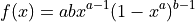
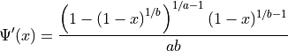
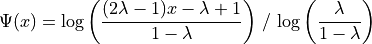
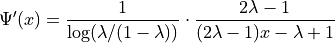
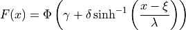
Denote by  the one-dimensional PDF,
  the
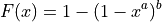
one-dimensional CDF, and
the
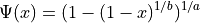
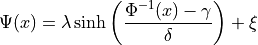
one-dimensional CDF, and  the inverse CDF transform
that takes samples mimicking
the inverse CDF transform
that takes samples mimicking ![\mathcal{U}[0,1]](../_images/math/d353aaa9c632654180ff3585fdda27778da89039.png) to mimic the
desired one-dimensional true measure. For each of these true measures we
assume the dimensions are independent, so the density and CDF and
computed by taking the product across dimensions and the inverse
transform is applied elementwise.
to mimic the
desired one-dimensional true measure. For each of these true measures we
assume the dimensions are independent, so the density and CDF and
computed by taking the product across dimensions and the inverse
transform is applied elementwise.
Parameters 
Parameter 
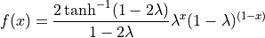
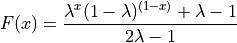
If  , then
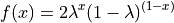


If  , then
Johnson’s :math:`S_U <https://en.wikipedia.org/wiki/Johnson%27s_SU-distribution>`__
Parameters 
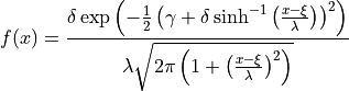
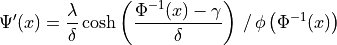
where  is the standard normal PDF and
  is the
standard normal CDF.
is the
standard normal CDF.
Imports
from qmcpy import *
from scipy.special import gamma
from numpy import *
import matplotlib
from matplotlib import pyplot
%matplotlib inline
pyplot.rc('font', size=16)          # controls default text sizes
pyplot.rc('axes', titlesize=16)     # fontsize of the axes title
pyplot.rc('axes', labelsize=16)     # fontsize of the x and y labels
pyplot.rc('xtick', labelsize=16)    # fontsize of the tick labels
pyplot.rc('ytick', labelsize=16)    # fontsize of the tick labels
pyplot.rc('legend', fontsize=16)    # legend fontsize
pyplot.rc('figure', titlesize=16)   # fontsize of the figure title
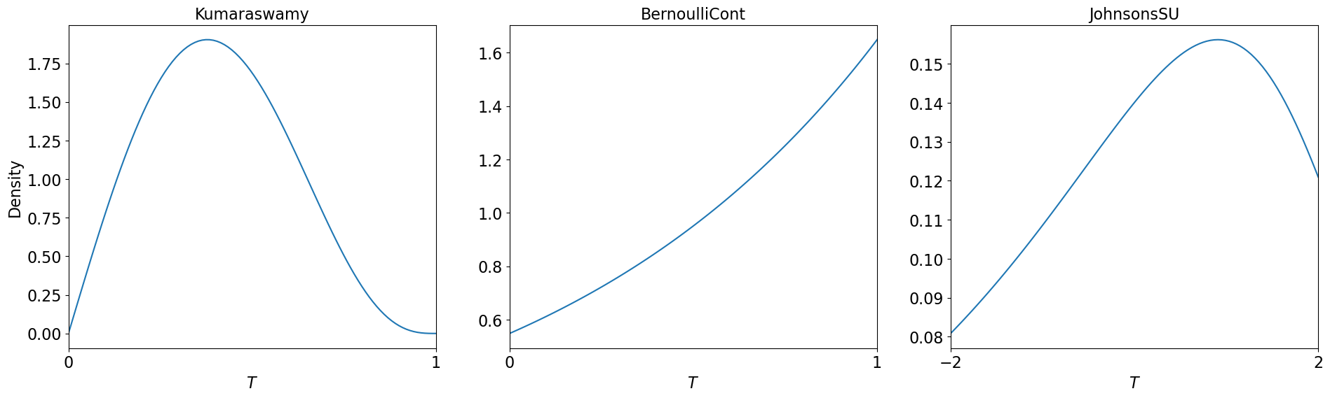
1D Density Plot
def plt_1d(tm,lim,ax):
    print(tm)
    n_mesh = 100
    ticks = linspace(*lim,n_mesh)
    y = tm._weight(ticks[:,None])
    ax.plot(ticks,y)
    ax.set_xlim(lim)
    ax.set_xlabel("$T$")
    ax.set_xticks(lim)
    ax.set_title(type(tm).__name__)
fig,ax = pyplot.subplots(figsize=(23,6),nrows=1,ncols=3)
sobol = Sobol(1)
kumaraswamy = Kumaraswamy(sobol,a=2,b=4)
plt_1d(kumaraswamy,lim=[0,1],ax=ax[0])
bern = BernoulliCont(sobol,lam=.75)
plt_1d(bern,lim=[0,1],ax=ax[1])
jsu = JohnsonsSU(sobol,gamma=1,xi=2,delta=1,lam=2)
plt_1d(jsu,lim=[-2,2],ax=ax[2])
ax[0].set_ylabel("Density");
Kumaraswamy (TrueMeasure Object)
    a               2^(1)
    b               2^(2)
BernoulliCont (TrueMeasure Object)
    lam             0.750
JohnsonsSU (TrueMeasure Object)
    gamma           1
    xi              2^(1)
    delta           1
    lam             2^(1)
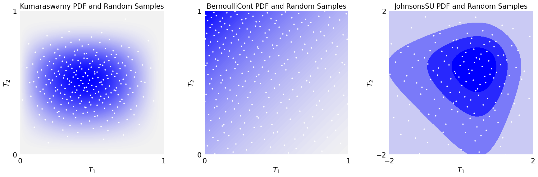
2D Density Plot
def plt_2d(tm,n,lim,ax):
    print(tm)
    n_mesh = 502
    # Points
    t = tm.gen_samples(n)
    # PDF
    mesh = zeros(((n_mesh)**2,3),dtype=float)
    grid_tics = linspace(*lim,n_mesh)
    x_mesh,y_mesh = meshgrid(grid_tics,grid_tics)
    mesh[:,0] = x_mesh.flatten()
    mesh[:,1] = y_mesh.flatten()
    mesh[:,2] = tm._weight(mesh[:,:2])
    z_mesh = mesh[:,2].reshape((n_mesh,n_mesh))
    #   colors
    clevel = arange(mesh[:,2].min(),mesh[:,2].max(),.025)
    cmap = matplotlib.colors.LinearSegmentedColormap.from_list("", [(.95,.95,.95),(0,0,1)])
    # cmap = pyplot.get_cmap('Blues')
    #   contour + scatter plot
    ax.contourf(x_mesh,y_mesh,z_mesh,clevel,cmap=cmap,extend='both')
    ax.scatter(t[:,0],t[:,1],s=5,color='w')
    #   axis
    for nsew in ['top','bottom','left','right']: ax.spines[nsew].set_visible(False)
    ax.xaxis.set_ticks_position('none')
    ax.yaxis.set_ticks_position('none')
    ax.set_aspect(1)
    ax.set_xlim(lim)
    ax.set_xticks(lim)
    ax.set_ylim(lim)
    ax.set_yticks(lim)
    #   labels
    ax.set_xlabel('$T_1$')
    ax.set_ylabel('$T_2$')
    ax.set_title('%s PDF and Random Samples'%type(tm).__name__)
    #   metas
    fig.tight_layout()
fig,ax = pyplot.subplots(figsize=(18,6),nrows=1,ncols=3)
sobol = Sobol(2)
kumaraswamy = Kumaraswamy(sobol,a=[2,3],b=[3,5])
plt_2d(kumaraswamy,n=2**8,lim=[0,1],ax=ax[0])
bern = BernoulliCont(sobol,lam=[.25,.75])
plt_2d(bern,n=2**8,lim=[0,1],ax=ax[1])
jsu = JohnsonsSU(sobol,gamma=[1,1],xi=[1,1],delta=[1,1],lam=[1,1])
plt_2d(jsu,n=2**8,lim=[-2,2],ax=ax[2])
Kumaraswamy (TrueMeasure Object)
    a               [2 3]
    b               [3 5]
BernoulliCont (TrueMeasure Object)
    lam             [0.25 0.75]
JohnsonsSU (TrueMeasure Object)
    gamma           [1 1]
    xi              [1 1]
    delta           [1 1]
    lam             [1 1]
1D Expected Values
def compute_expected_val(tm,true_value,abs_tol):
    if tm.d!=1: raise Exception("tm must be 1 dimensional for this test")
    cf = CustomFun(tm, g=lambda x:x)
    sol,data = CubQMCSobolG(cf,abs_tol=abs_tol).integrate()
    error = abs(true_value-sol)
    if error>abs_tol:
        raise Exception("QMC error %.3f not within tolerance."%error)
    print("%s integration within tolerance"%type(tm).__name__)
    print("\tEstimated mean: %.4f"%sol)
    print("\t%s"%str(tm).replace('\n','\n\t'))
abs_tol = 1e-5
# kumaraswamy
a,b = 2,6
kuma = Kumaraswamy(Sobol(1),a,b)
kuma_tv = b*gamma(1+1/a)*gamma(b)/gamma(1+1/a+b)
compute_expected_val(kuma,kuma_tv,abs_tol)
# Continuous Bernoulli
lam = .75
bern = BernoulliCont(Sobol(1),lam=lam)
bern_tv = 1/2 if lam==1/2 else lam/(2*lam-1)+1/(2*arctanh(1-2*lam))
compute_expected_val(bern,bern_tv,abs_tol)
# Johnson's SU
_gamma,xi,delta,lam = 1,2,3,4
jsu = JohnsonsSU(Sobol(1),gamma=_gamma,xi=xi,delta=delta,lam=lam)
jsu_tv = xi-lam*exp(1/(2*delta**2))*sinh(_gamma/delta)
compute_expected_val(jsu,jsu_tv,abs_tol)
Kumaraswamy integration within tolerance
    Estimated mean: 0.3410
    Kumaraswamy (TrueMeasure Object)
        a               2^(1)
        b               6
BernoulliCont integration within tolerance
    Estimated mean: 0.5898
    BernoulliCont (TrueMeasure Object)
        lam             0.750
JohnsonsSU integration within tolerance
    Estimated mean: 0.5642
    JohnsonsSU (TrueMeasure Object)
        gamma           1
        xi              2^(1)
        delta           3
        lam             2^(2)
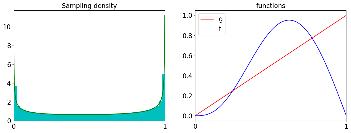
Importance Sampling with a Single Kumaraswamy
# compose with a Kumaraswamy transformation
abs_tol = 1e-4
cf = CustomFun(Uniform(Kumaraswamy(Sobol(1,seed=7),a=.5,b=.5)), g=lambda x:x)
sol,data = CubQMCSobolG(cf,abs_tol=abs_tol).integrate()
print(data)
true_val = .5 # expected value of standard uniform
error = abs(true_val-sol)
if error>abs_tol: raise Exception("QMC error %.3f not within tolerance."%error)
LDTransformData (AccumulateData Object)
    solution        0.500
    comb_bound_low  0.500
    comb_bound_high 0.500
    comb_flags      1
    n_total         2^(11)
    n               2^(11)
    time_integrate  0.012
CubQMCSobolG (StoppingCriterion Object)
    abs_tol         1.00e-04
    rel_tol         0
    n_init          2^(10)
    n_max           2^(35)
CustomFun (Integrand Object)
Uniform (TrueMeasure Object)
    lower_bound     0
    upper_bound     1
    transform       Kumaraswamy (TrueMeasure Object)
                       a               2^(-1)
                       b               2^(-1)
Sobol (DiscreteDistribution Object)
    d               1
    dvec            0
    randomize       LMS_DS
    graycode        0
    entropy         7
    spawn_key       ()
# plot the above functions
x = linspace(0,1,1000).reshape(-1,1)
x = x[1:-1] # plotting locations
# plot
fig,ax = pyplot.subplots(ncols=2,figsize=(15,5))
#    density
rho = cf.true_measure.transform._weight(x)
tfvals = cf.true_measure.transform._transform_r(x)
ax[0].hist(tfvals,density=True,bins=50,color='c')
ax[0].plot(x,rho,color='g',linewidth=2)
ax[0].set_title('Sampling density')
#    functions
gs = cf.g(x)
fs = cf.f(x)
ax[1].plot(x,gs,color='r',label='g')
ax[1].plot(x,fs,color='b',label='f')
ax[1].legend()
ax[1].set_title('functions');
# metas
for i in range(2):
    ax[i].set_xlim([0,1])
    ax[i].set_xticks([0,1])
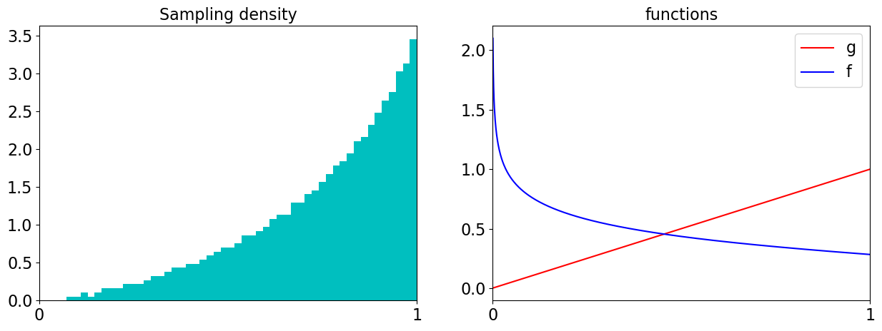
Importance Sampling with 2 (Composed) Kumaraswamys
# compose multiple Kumaraswamy distributions
abs_tol = 1e-3
dd = Sobol(1,seed=7)
t1 = Kumaraswamy(dd,a=.5,b=.5) # first transformation
t2 = Kumaraswamy(t1,a=5,b=2) # second transformation
cf = CustomFun(Uniform(t2), g=lambda x:x)
sol,data = CubQMCSobolG(cf,abs_tol=abs_tol).integrate() # expected value of standard uniform
print(data)
true_val = .5
error = abs(true_val-sol)
if error>abs_tol: raise Exception("QMC error %.3f not within tolerance."%error)
LDTransformData (AccumulateData Object)
    solution        0.500
    comb_bound_low  0.499
    comb_bound_high 0.501
    comb_flags      1
    n_total         2^(10)
    n               2^(10)
    time_integrate  0.007
CubQMCSobolG (StoppingCriterion Object)
    abs_tol         0.001
    rel_tol         0
    n_init          2^(10)
    n_max           2^(35)
CustomFun (Integrand Object)
Uniform (TrueMeasure Object)
    lower_bound     0
    upper_bound     1
    transform       Kumaraswamy (TrueMeasure Object)
                       a               5
                       b               2^(1)
                       transform       Kumaraswamy (TrueMeasure Object)
                                          a               2^(-1)
                                          b               2^(-1)
Sobol (DiscreteDistribution Object)
    d               1
    dvec            0
    randomize       LMS_DS
    graycode        0
    entropy         7
    spawn_key       ()
x = linspace(0,1,1000).reshape(-1,1)
x = x[1:-1] # plotting locations
# plot
fig,ax = pyplot.subplots(ncols=2,figsize=(15,5))
#    density
tfvals = cf.true_measure.transform._transform_r(x)
ax[0].hist(tfvals,density=True,bins=50,color='c')
ax[0].set_title('Sampling density')
#    functions
gs = cf.g(x)
fs = cf.f(x)
ax[1].plot(x,gs,color='r',label='g')
ax[1].plot(x,fs,color='b',label='f')
ax[1].legend()
for i in range(2):
    ax[i].set_xlim([0,1])
    ax[i].set_xticks([0,1])
ax[1].set_title('functions');
Can we Improve the Keister function?
abs_tol = 1e-4
d = 1
# standard method
keister_std = Keister(Sobol(d))
sol_std,data_std = CubQMCSobolG(keister_std,abs_tol=abs_tol).integrate()
print("Standard method estimate of %.4f took %.2e seconds and %.2e samples"%\
      (sol_std,data_std.time_integrate,data_std.n_total))
print(keister_std.true_measure)
Standard method estimate of 1.3804 took 1.20e-02 seconds and 1.64e+04 samples
Gaussian (TrueMeasure Object)
    mean            0
    covariance      2^(-1)
    decomp_type     PCA
# Kumaraswamy importance sampling
dd = Sobol(d,seed=7)
t1 = Kumaraswamy(dd,a=.8,b=.8) # first transformation
t2 = Gaussian(t1)
keister_kuma = Keister(t2)
sol_kuma,data_kuma = CubQMCSobolG(keister_kuma,abs_tol=abs_tol).integrate()
print("Kumaraswamy IS estimate of %.4f took %.2e seconds and %.2e samples"%\
      (sol_kuma,data_kuma.time_integrate,data_kuma.n_total))
t_frac = data_kuma.time_integrate/data_std.time_integrate
n_frac = data_kuma.n_total/data_std.n_total
print('That is %.1f%% of the time and %.1f%% of the samples compared to default keister.'%(t_frac*100,n_frac*100))
print(keister_kuma.true_measure)
Kumaraswamy IS estimate of 1.3804 took 1.21e-02 seconds and 2.05e+03 samples
That is 100.9% of the time and 12.5% of the samples compared to default keister.
Gaussian (TrueMeasure Object)
    mean            0
    covariance      2^(-1)
    decomp_type     PCA
    transform       Gaussian (TrueMeasure Object)
                       mean            0
                       covariance      1
                       decomp_type     PCA
                       transform       Kumaraswamy (TrueMeasure Object)
                                          a               0.800
                                          b               0.800
# Continuous Bernoulli importance sampling
dd = Sobol(d,seed=7)
t1 = BernoulliCont(dd,lam=.25) # first transformation
#t2 = BernoulliCont(t1,lam=.75) # first transformation
t3 = Gaussian(t1)
keister_cb = Keister(t3)
sol_cb,data_cb = CubQMCSobolG(keister_cb,abs_tol=abs_tol).integrate()
print("Continuous Bernoulli IS estimate of %.4f took %.2e seconds and %.2e samples"%\
      (sol_cb,data_cb.time_integrate,data_cb.n_total))
t_frac = data_cb.time_integrate/data_std.time_integrate
n_frac = data_cb.n_total/data_std.n_total
print('That is %.1f%% of the time and %.1f%% of the samples compared to default keister.'%(t_frac*100,n_frac*100))
print(keister_cb.true_measure)
Continuous Bernoulli IS estimate of 1.3804 took 4.15e-02 seconds and 8.19e+03 samples
That is 346.8% of the time and 50.0% of the samples compared to default keister.
Gaussian (TrueMeasure Object)
    mean            0
    covariance      2^(-1)
    decomp_type     PCA
    transform       Gaussian (TrueMeasure Object)
                       mean            0
                       covariance      1
                       decomp_type     PCA
                       transform       BernoulliCont (TrueMeasure Object)
                                          lam             2^(-2)
#  Kumaraswamy importance sampling
dd = Sobol(d,seed=7)
t1 = JohnsonsSU(dd,xi=2,delta=1,gamma=2,lam=1) # first transformation
keister_jsu = Keister(t1)
sol_jsu,data_jsu = CubQMCSobolG(keister_jsu,abs_tol=abs_tol).integrate()
print("Kumaraswamy IS estimate of %.4f took %.2e seconds and %.2e samples"%\
      (sol_jsu,data_jsu.time_integrate,data_jsu.n_total))
t_frac = data_jsu.time_integrate/data_std.time_integrate
n_frac = data_jsu.n_total/data_std.n_total
print('That is %.1f%% of the time and %.1f%% of the samples compared to default keister.'%(t_frac*100,n_frac*100))
print(keister_jsu.true_measure)
Kumaraswamy IS estimate of 1.3804 took 4.08e-02 seconds and 8.19e+03 samples
That is 340.9% of the time and 50.0% of the samples compared to default keister.
Gaussian (TrueMeasure Object)
    mean            0
    covariance      2^(-1)
    decomp_type     PCA
    transform       JohnsonsSU (TrueMeasure Object)
                       gamma           2^(1)
                       xi              2^(1)
                       delta           1
                       lam             1
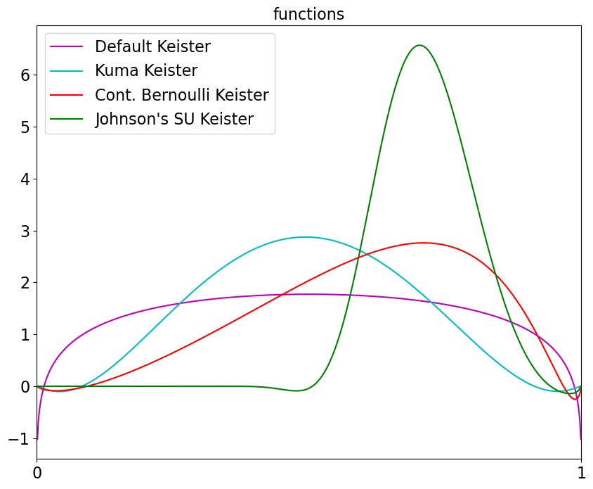
x = linspace(0,1,1000).reshape(-1,1)
x = x[1:-1] # plotting locations
# plot
fig,ax = pyplot.subplots(figsize=(10,8))
#    functions
fs = [keister_std.f,keister_kuma.f,keister_cb.f,keister_jsu.f]
labels = ['Default Keister','Kuma Keister','Cont. Bernoulli Keister',"Johnson's SU Keister"]
colors = ['m','c','r','g']
for f,label,color in zip(fs,labels,colors): ax.plot(x,f(x),color=color,label=label)
ax.legend()
ax.set_xlim([0,1])
ax.set_xticks([0,1])
ax.set_title('functions');