QMCPy Documentation

_images/discrete_distribution_overview.png

Discrete Distribution Class

_images/discrete_distribution_specific.png

Abstract Discrete Distribution Class

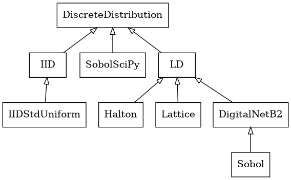
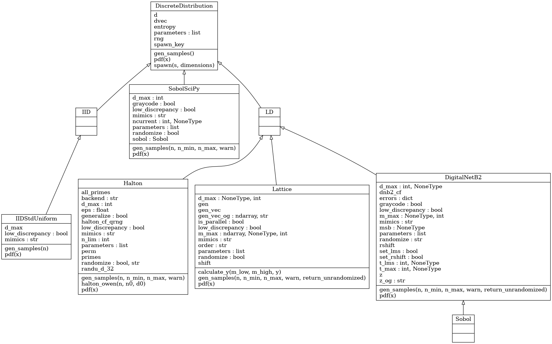
class qmcpy.discrete_distribution._discrete_distribution.DiscreteDistribution(dimension, seed)

Discrete Distribution abstract class. DO NOT INSTANTIATE.

__init__(dimension, seed)

Parameters

dimension (int or ndarray) – dimension of the generator. If an int is passed in, use sequence dimensions [0,…,dimensions-1]. If a ndarray is passed in, use these dimension indices in the sequence. Note that this is not relevant for IID generators.
seed (int or numpy.random.SeedSequence) – seed to create random number generator

gen_samples(*args)

ABSTRACT METHOD to generate samples from this discrete distribution.

Parameters: args (tuple) – tuple of positional argument. See implementations for details
Returns: n x d array of samples
Return type: ndarray

pdf(x): ABSTRACT METHOD to evaluate pdf of distribution the samples mimic at locations of x.

spawn(s=1, dimensions=None)

Spawn new instances of the current discrete distribution but with new seeds and dimensions. Developed for multi-level and multi-replication (Q)MC algorithms.

Parameters

s (int) – number of spawn
dimensions (ndarray) – length s array of dimension for each spawn. Defaults to current dimension

Returns

list of DiscreteDistribution instances with new seeds and dimensions

Return type

list

class qmcpy.discrete_distribution._discrete_distribution.IID(dimension, seed)

class qmcpy.discrete_distribution._discrete_distribution.LD(dimension, seed)

Digital Net Base 2

class qmcpy.discrete_distribution.digital_net_b2.digital_net_b2.DigitalNetB2(dimension=1, randomize='LMS_DS', graycode=False, seed=None, generating_matrices='sobol_mat.21201.32.32.msb.npy', d_max=None, t_max=None, m_max=None, msb=None, t_lms=None, _verbose=False)

Quasi-Random digital nets in base 2.

>>> dnb2 = DigitalNetB2(2,seed=7)
>>> dnb2.gen_samples(4)
array([[0.56269008, 0.17377997],
       [0.346653  , 0.65070632],
       [0.82074548, 0.95490574],
       [0.10422261, 0.49458097]])
>>> dnb2.gen_samples(1)
array([[0.56269008, 0.17377997]])
>>> dnb2
DigitalNetB2 (DiscreteDistribution Object)
    d               2^(1)
    dvec            [0 1]
    randomize       LMS_DS
    graycode        0
    entropy         7
    spawn_key       ()
>>> DigitalNetB2(dimension=2,randomize=False,graycode=True).gen_samples(n_min=2,n_max=4)
array([[0.75, 0.25],
       [0.25, 0.75]])
>>> DigitalNetB2(dimension=2,randomize=False,graycode=False).gen_samples(n_min=2,n_max=4)
array([[0.25, 0.75],
       [0.75, 0.25]])
>>> dnb2_alpha2 = DigitalNetB2(5,randomize=False,generating_matrices='sobol_mat_alpha2.10600.64.32.lsb.npy')
>>> dnb2_alpha2.gen_samples(8,warn=False)
array([[0.      , 0.      , 0.      , 0.      , 0.      ],
       [0.75    , 0.75    , 0.75    , 0.75    , 0.75    ],
       [0.4375  , 0.9375  , 0.1875  , 0.6875  , 0.1875  ],
       [0.6875  , 0.1875  , 0.9375  , 0.4375  , 0.9375  ],
       [0.296875, 0.171875, 0.109375, 0.796875, 0.859375],
       [0.546875, 0.921875, 0.859375, 0.046875, 0.109375],
       [0.234375, 0.859375, 0.171875, 0.484375, 0.921875],
       [0.984375, 0.109375, 0.921875, 0.734375, 0.171875]])

References

[1] Marius Hofert and Christiane Lemieux (2019). qrng: (Randomized) Quasi-Random Number Generators. R package version 0.0-7. https://CRAN.R-project.org/package=qrng.

[2] Faure, Henri, and Christiane Lemieux. “Implementation of Irreducible Sobol’ Sequences in Prime Power Bases.” Mathematics and Computers in Simulation 161 (2019): 13-22. Crossref. Web.

[3] F.Y. Kuo & D. Nuyens. Application of quasi-Monte Carlo methods to elliptic PDEs with random diffusion coefficients - a survey of analysis and implementation, Foundations of Computational Mathematics, 16(6):1631-1696, 2016. springer link: https://link.springer.com/article/10.1007/s10208-016-9329-5 arxiv link: https://arxiv.org/abs/1606.06613

[4] D. Nuyens, The Magic Point Shop of QMC point generators and generating vectors. MATLAB and Python software, 2018. Available from https://people.cs.kuleuven.be/~dirk.nuyens/ https://bitbucket.org/dnuyens/qmc-generators/src/cb0f2fb10fa9c9f2665e41419097781b611daa1e/cpp/digitalseq_b2g.hpp

[5] Paszke, A., Gross, S., Massa, F., Lerer, A., Bradbury, J., Chanan, G., … Chintala, S. (2019). PyTorch: An Imperative Style, High-Performance Deep Learning Library. In H. Wallach, H. Larochelle, A. Beygelzimer, F. d extquotesingle Alch'e-Buc, E. Fox, & R. Garnett (Eds.), Advances in Neural Information Processing Systems 32 (pp. 8024-8035). Curran Associates, Inc. Retrieved from http://papers.neurips.cc/paper/9015-pytorch-an-imperative-style-high-performance-deep-learning-library.pdf

[6] I.M. Sobol’, V.I. Turchaninov, Yu.L. Levitan, B.V. Shukhman: “Quasi-Random Sequence Generators” Keldysh Institute of Applied Mathematics, Russian Acamdey of Sciences, Moscow (1992).

[7] Sobol, Ilya & Asotsky, Danil & Kreinin, Alexander & Kucherenko, Sergei. (2011). Construction and Comparison of High-Dimensional Sobol’ Generators. Wilmott. 2011. 10.1002/wilm.10056.

[8] Paul Bratley and Bennett L. Fox. 1988. Algorithm 659: Implementing Sobol’s quasirandom sequence generator. ACM Trans. Math. Softw. 14, 1 (March 1988), 88-100. DOI:https://doi.org/10.1145/42288.214372

__init__(dimension=1, randomize='LMS_DS', graycode=False, seed=None, generating_matrices='sobol_mat.21201.32.32.msb.npy', d_max=None, t_max=None, m_max=None, msb=None, t_lms=None, _verbose=False)

Parameters

dimension (int or ndarray) – dimension of the generator. If an int is passed in, use sequence dimensions [0,…,dimensions-1]. If a ndarray is passed in, use these dimension indices in the sequence.
randomize (bool) – apply randomization? True defaults to LMS_DS. Can also explicitly pass in ‘LMS_DS’: linear matrix scramble with digital shift ‘LMS’: linear matrix scramble only ‘DS’: digital shift only
graycode (bool) – indicator to use graycode ordering (True) or natural ordering (False)
seed (list) – int seed of list of seeds, one for each dimension.
generating_matrices (ndarray or str) – generating matrices or path to generating matrices. ndarray should have shape (d_max, m_max) where each int has t_max bits generating_matrices should be formatted like gen_mat.21201.32.32.msb.npy with name.d_max.t_max.m_max.{msb,lsb}.npy
d_max (int) – max dimension
t_max (int) – number of bits in each int of each generating matrix. aka: number of rows in a generating matrix with ints expanded into columns
m_max (int) – 2^m_max is the number of samples supported. aka: number of columns in a generating matrix with ints expanded into columns
msb (bool) – bit storage as ints. e.g. if t_max=3, then 6 is [1 1 0] in MSB (True) and [0 1 1] in LSB (False)
t_lms (int) – LMS scrambling matrix will be t_lms x t_max for generating matrix of shape t_max x m_max
_verbose (bool) – print randomization details

gen_samples(n=None, n_min=0, n_max=8, warn=True, return_unrandomized=False)

Generate samples

Parameters

n (int) – if n is supplied, generate from n_min=0 to n_max=n samples. Otherwise use the n_min and n_max explicitly supplied as the following 2 arguments
n_min (int) – Starting index of sequence.
n_max (int) – Final index of sequence.
return_unrandomized (bool) – return unrandomized samples as well? If True, return randomized_samples,unrandomized_samples. Note that this only applies when randomize includes Digital Shift. Also note that unrandomized samples included linear matrix scrambling if applicable.

Returns

(n_max-n_min) x d (dimension) array of samples

Return type

ndarray

pdf(x): pdf of a standard uniform

class qmcpy.discrete_distribution.digital_net_b2.digital_net_b2.Sobol(dimension=1, randomize='LMS_DS', graycode=False, seed=None, generating_matrices='sobol_mat.21201.32.32.msb.npy', d_max=None, t_max=None, m_max=None, msb=None, t_lms=None, _verbose=False)

Lattice

class qmcpy.discrete_distribution.lattice.lattice.Lattice(dimension=1, randomize=True, order='natural', seed=None, generating_vector='lattice_vec.3600.20.npy', d_max=None, m_max=None, is_parallel=True)

Quasi-Random Lattice nets in base 2.

>>> l = Lattice(2,seed=7)
>>> l.gen_samples(4)
array([[0.04386058, 0.58727432],
       [0.54386058, 0.08727432],
       [0.29386058, 0.33727432],
       [0.79386058, 0.83727432]])
>>> l.gen_samples(1)
array([[0.04386058, 0.58727432]])
>>> l
Lattice (DiscreteDistribution Object)
    d               2^(1)
    dvec            [0 1]
    randomize       1
    order           natural
    gen_vec         [     1 182667]
    entropy         7
    spawn_key       ()
>>> Lattice(dimension=2,randomize=False,order='natural').gen_samples(4, warn=False)
array([[0.  , 0.  ],
       [0.5 , 0.5 ],
       [0.25, 0.75],
       [0.75, 0.25]])
>>> Lattice(dimension=2,randomize=False,order='linear').gen_samples(4, warn=False)
array([[0.  , 0.  ],
       [0.25, 0.75],
       [0.5 , 0.5 ],
       [0.75, 0.25]])
>>> Lattice(dimension=2,randomize=False,order='mps').gen_samples(4, warn=False)
array([[0.  , 0.  ],
       [0.5 , 0.5 ],
       [0.25, 0.75],
       [0.75, 0.25]])
>>> l = Lattice(2,generating_vector=25,seed=55)
>>> l.gen_samples(4)
array([[0.84489224, 0.30534549],
       [0.34489224, 0.80534549],
       [0.09489224, 0.05534549],
       [0.59489224, 0.55534549]])
>>> l
Lattice (DiscreteDistribution Object)
    d               2^(1)
    dvec            [0 1]
    randomize       1
    order           natural
    gen_vec         [       1 11961679]
    entropy         55
    spawn_key       ()
>>> Lattice(dimension=4,randomize=False,seed=353,generating_vector=26).gen_samples(8,warn=False)
array([[0.   , 0.   , 0.   , 0.   ],
       [0.5  , 0.5  , 0.5  , 0.5  ],
       [0.25 , 0.25 , 0.75 , 0.75 ],
       [0.75 , 0.75 , 0.25 , 0.25 ],
       [0.125, 0.125, 0.875, 0.875],
       [0.625, 0.625, 0.375, 0.375],
       [0.375, 0.375, 0.625, 0.625],
       [0.875, 0.875, 0.125, 0.125]])
>>> Lattice(dimension=4,randomize=False,seed=353,generating_vector=26,is_parallel=True).gen_samples(8,warn=False)
array([[0.   , 0.   , 0.   , 0.   ],
       [0.5  , 0.5  , 0.5  , 0.5  ],
       [0.25 , 0.25 , 0.75 , 0.75 ],
       [0.75 , 0.75 , 0.25 , 0.25 ],
       [0.125, 0.125, 0.875, 0.875],
       [0.625, 0.625, 0.375, 0.375],
       [0.375, 0.375, 0.625, 0.625],
       [0.875, 0.875, 0.125, 0.125]])

References

[1] Sou-Cheng T. Choi, Yuhan Ding, Fred J. Hickernell, Lan Jiang, Lluis Antoni Jimenez Rugama, Da Li, Jagadeeswaran Rathinavel, Xin Tong, Kan Zhang, Yizhi Zhang, and Xuan Zhou, GAIL: Guaranteed Automatic Integration Library (Version 2.3) [MATLAB Software], 2019. Available from http://gailgithub.github.io/GAIL_Dev/

[2] F.Y. Kuo & D. Nuyens. Application of quasi-Monte Carlo methods to elliptic PDEs with random diffusion coefficients - a survey of analysis and implementation, Foundations of Computational Mathematics, 16(6):1631-1696, 2016. springer link: https://link.springer.com/article/10.1007/s10208-016-9329-5 arxiv link: https://arxiv.org/abs/1606.06613

[3] D. Nuyens, The Magic Point Shop of QMC point generators and generating vectors. MATLAB and Python software, 2018. Available from https://people.cs.kuleuven.be/~dirk.nuyens/

[4] Constructing embedded lattice rules for multivariate integration R Cools, FY Kuo, D Nuyens - SIAM J. Sci. Comput., 28(6), 2162-2188.

[5] L’Ecuyer, Pierre & Munger, David. (2015). LatticeBuilder: A General Software Tool for Constructing Rank-1 Lattice Rules. ACM Transactions on Mathematical Software. 42. 10.1145/2754929.

__init__(dimension=1, randomize=True, order='natural', seed=None, generating_vector='lattice_vec.3600.20.npy', d_max=None, m_max=None, is_parallel=True)

Parameters

dimension (int or ndarray) – dimension of the generator. If an int is passed in, use sequence dimensions [0,…,dimensions-1]. If a ndarray is passed in, use these dimension indices in the sequence.
randomize (bool) – If True, apply shift to generated samples. Note: Non-randomized lattice sequence includes the origin.
order (str) – ‘linear’, ‘natural’, or ‘mps’ ordering.
seed (None or int or numpy.random.SeedSeq) – seed the random number generator for reproducibility
generating_vector (ndarray, str or int) – generating matrix or path to generating matrices. ndarray should have shape (d_max). a string generating_vector should be formatted like ‘lattice_vec.3600.20.npy’ where ‘name.d_max.m_max.npy’ an integer should be an odd larger than 1; passing an integer M would create a random generating vector supporting up to 2^M points. M is restricted between 2 and 26 for numerical percision. The generating vector is [1,v_1,v_2,…,v_dimension], where v_i is an integer in {3,5,…,2*M-1}.
d_max (int) – maximum dimension
m_max (int) – 2^m_max is the max number of supported samples
is_parallel (bool) – Default to True to perform parallel computations, False serial

Note

d_max and m_max are required if generating_vector is a ndarray. If generating_vector is an string (path), d_max and m_max can be taken from the file name if None

gen_samples(n=None, n_min=0, n_max=8, warn=True, return_unrandomized=False)

Generate lattice samples

Parameters

n (int) – if n is supplied, generate from n_min=0 to n_max=n samples. Otherwise use the n_min and n_max explicitly supplied as the following 2 arguments
n_min (int) – Starting index of sequence.
n_max (int) – Final index of sequence.
return_unrandomized (bool) – return samples without randomization as 2nd return value. Will not be returned if randomize=False.

Returns

(n_max-n_min) x d (dimension) array of samples

Return type

ndarray

Note

Lattice generates in blocks from 2**m to 2**(m+1) so generating n_min=3 to n_max=9 requires necessarily produces samples from n_min=2 to n_max=16 and automatically subsets. May be inefficient for non-powers-of-2 samples sizes.

pdf(x): pdf of a standard uniform

Halton

class qmcpy.discrete_distribution.halton.Halton(dimension=1, randomize=True, generalize=True, seed=None)

Quasi-Random Halton nets.

>>> h_qrng = Halton(2,randomize='QRNG',generalize=True,seed=7)
>>> h_qrng.gen_samples(4)
array([[0.35362988, 0.38733489],
       [0.85362988, 0.72066823],
       [0.10362988, 0.05400156],
       [0.60362988, 0.498446  ]])
>>> h_qrng.gen_samples(1)
array([[0.35362988, 0.38733489]])
>>> h_qrng
Halton (DiscreteDistribution Object)
    d               2^(1)
    dvec            [0 1]
    randomize       QRNG
    generalize      1
    entropy         7
    spawn_key       ()
>>> h_owen = Halton(2,randomize='OWEN',generalize=False,seed=7)
>>> h_owen.gen_samples(4)
array([[0.64637012, 0.48226667],
       [0.14637012, 0.81560001],
       [0.89637012, 0.14893334],
       [0.39637012, 0.59337779]])
>>> h_owen
Halton (DiscreteDistribution Object)
    d               2^(1)
    dvec            [0 1]
    randomize       OWEN
    generalize      0
    entropy         7
    spawn_key       ()

References

[1] Marius Hofert and Christiane Lemieux (2019). qrng: (Randomized) Quasi-Random Number Generators. R package version 0.0-7. https://CRAN.R-project.org/package=qrng.

[2] Owen, A. B. “A randomized Halton algorithm in R,” 2017. arXiv:1706.02808 [stat.CO]

__init__(dimension=1, randomize=True, generalize=True, seed=None)

Parameters

dimension (int or ndarray) – dimension of the generator. If an int is passed in, use sequence dimensions [0,…,dimensions-1]. If a ndarray is passed in, use these dimension indices in the sequence.
randomize (str/bool) – select randomization method from ‘QRNG” [1], (max dimension = 360, supports generalize=True, default if randomize=True) or ‘OWEN’ [2], (max dimension = 1000),
generalize (bool) – generalize flag, only applicable to the QRNG generator
seed (None or int or numpy.random.SeedSeq) – seed the random number generator for reproducibility

gen_samples(n=None, n_min=0, n_max=8, warn=True)

Generate samples

Parameters

n (int) – if n is supplied, generate from n_min=0 to n_max=n samples. Otherwise use the n_min and n_max explicitly supplied as the following 2 arguments
n_min (int) – Starting index of sequence.
n_max (int) – Final index of sequence.

Returns

(n_max-n_min) x d (dimension) array of samples

Return type

ndarray

halton_owen(n, n0, d0=0): see gen_samples method and [1] Owen, A. B.A randomized Halton algorithm in R2017. arXiv:1706.02808 [stat.CO].

pdf(x): ABSTRACT METHOD to evaluate pdf of distribution the samples mimic at locations of x.

IID Standard Uniform

class qmcpy.discrete_distribution.iid_std_uniform.IIDStdUniform(dimension=1, seed=None)

A wrapper around NumPy’s IID Standard Uniform generator numpy.random.rand.

>>> dd = IIDStdUniform(dimension=2,seed=7)
>>> dd.gen_samples(4)
array([[0.04386058, 0.58727432],
       [0.3691824 , 0.65212985],
       [0.69669968, 0.10605352],
       [0.63025643, 0.13630282]])
>>> dd
IIDStdUniform (DiscreteDistribution Object)
    d               2^(1)
    entropy         7
    spawn_key       ()

__init__(dimension=1, seed=None)

Parameters

dimension (int) – dimension of samples
seed (None or int or numpy.random.SeedSeq) – seed the random number generator for reproducibility

gen_samples(n)

Generate samples

Parameters: n (int) – Number of observations to generate
Returns: n x self.d array of samples
Return type: ndarray

pdf(x): ABSTRACT METHOD to evaluate pdf of distribution the samples mimic at locations of x.

True Measure Class

Abstract Measure Class

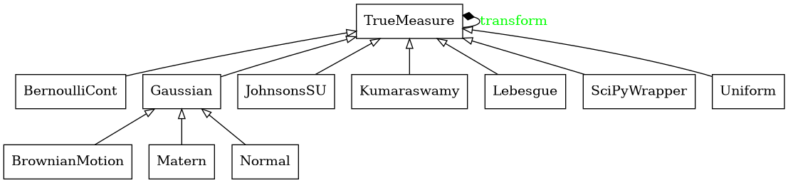
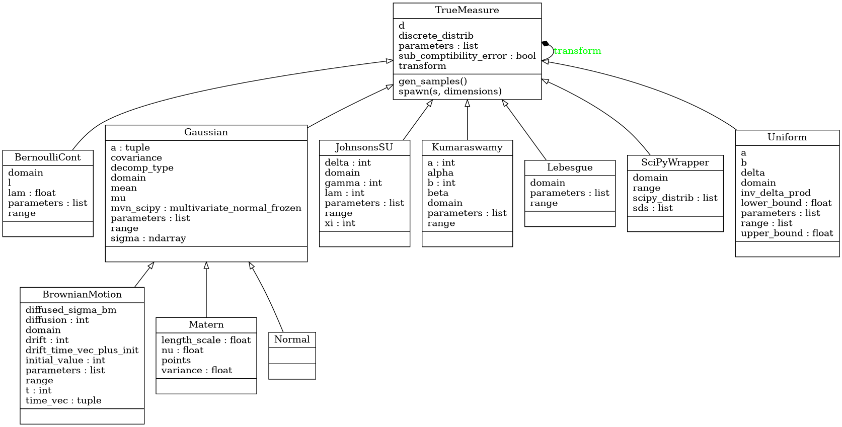
class qmcpy.true_measure._true_measure.TrueMeasure

True Measure abstract class. DO NOT INSTANTIATE.

gen_samples(*args, **kwargs)

Generate samples from the discrete distribution and transform them via the transform method.

Parameters

args (tuple) – positional arguments to the discrete distributions gen_samples method
kwargs (dict) – keyword arguments to the discrete distributions gen_samples method

Returns

n x d matrix of transformed samples

Return type

ndarray

spawn(s=1, dimensions=None)

Spawn new instances of the current discrete distribution but with new seeds and dimensions. Developed for multi-level and multi-replication (Q)MC algorithms.

Parameters

s (int) – number of spawn
dimensions (ndarray) – length s array of dimension for each spawn. Defaults to current dimension

Returns

list of TrueMeasures linked to newly spawned DiscreteDistributions

Return type

list

Uniform

class qmcpy.true_measure.uniform.Uniform(sampler, lower_bound=0.0, upper_bound=1.0)

>>> u = Uniform(DigitalNetB2(2,seed=7),lower_bound=[0,.5],upper_bound=[2,3])
>>> u.gen_samples(4)
array([[1.12538017, 0.93444992],
       [0.693306  , 2.12676579],
       [1.64149095, 2.88726434],
       [0.20844522, 1.73645241]])
>>> u
Uniform (TrueMeasure Object)
    lower_bound     [0.  0.5]
    upper_bound     [2 3]

__init__(sampler, lower_bound=0.0, upper_bound=1.0)

Parameters

sampler (DiscreteDistribution/TrueMeasure) – A discrete distribution from which to transform samples or a true measure by which to compose a transform
lower_bound (float) – a for Uniform(a,b)
upper_bound (float) – b for Uniform(a,b)

Gaussian

class qmcpy.true_measure.gaussian.Gaussian(sampler, mean=0.0, covariance=1.0, decomp_type='PCA')

Normal Measure.

>>> g = Gaussian(DigitalNetB2(2,seed=7),mean=[1,2],covariance=[[9,4],[4,5]])
>>> g.gen_samples(4)
array([[-0.23979685,  2.98944192],
       [ 2.45994002,  2.17853622],
       [-0.22923897, -1.92667105],
       [ 4.6127697 ,  4.25820377]])
>>> g
Gaussian (TrueMeasure Object)
    mean            [1 2]
    covariance      [[9 4]
                    [4 5]]
    decomp_type     PCA

__init__(sampler, mean=0.0, covariance=1.0, decomp_type='PCA')

Parameters

sampler (DiscreteDistribution/TrueMeasure) – A discrete distribution from which to transform samples or a true measure by which to compose a transform
mean (float) – mu for Normal(mu,sigma^2)
covariance (ndarray) – sigma^2 for Normal(mu,sigma^2). A float or d (dimension) vector input will be extended to covariance*eye(d)
decomp_type (str) – method of decomposition either “PCA” for principal component analysis or “Cholesky” for cholesky decomposition.

class qmcpy.true_measure.gaussian.Normal(sampler, mean=0.0, covariance=1.0, decomp_type='PCA')

Brownian Motion

class qmcpy.true_measure.brownian_motion.BrownianMotion(sampler, t_final=1, initial_value=0, drift=0, diffusion=1, decomp_type='PCA')

Geometric Brownian Motion.

>>> bm = BrownianMotion(DigitalNetB2(4,seed=7),t_final=2,drift=2)
>>> bm.gen_samples(2)
array([[0.44018403, 1.62690477, 2.69418273, 4.21753174],
       [1.97549563, 2.27002956, 2.92802765, 4.77126959]])
>>> bm
BrownianMotion (TrueMeasure Object)
    time_vec        [0.5 1.  1.5 2. ]
    drift           2^(1)
    mean            [1. 2. 3. 4.]
    covariance      [[0.5 0.5 0.5 0.5]
                    [0.5 1.  1.  1. ]
                    [0.5 1.  1.5 1.5]
                    [0.5 1.  1.5 2. ]]
    decomp_type     PCA

__init__(sampler, t_final=1, initial_value=0, drift=0, diffusion=1, decomp_type='PCA')

BrowianMotion(t) = (initial_value) + (drift)*t + sqrt{diffusion}*StandardBrownianMotion(t)

Parameters

sampler (DiscreteDistribution/TrueMeasure) – A discrete distribution from which to transform samples or a true measure by which to compose a transform
t_final (float) – end time for the Brownian Motion.
initial_value (float) – See above formula
drift (int) – See above formula
diffusion (int) – See above formula
decomp_type (str) – method of decomposition either “PCA” for principal component analysis or “Cholesky” for cholesky decomposition.

Lebesgue

class qmcpy.true_measure.lebesgue.Lebesgue(sampler)

>>> Lebesgue(Gaussian(DigitalNetB2(2,seed=7)))
Lebesgue (TrueMeasure Object)
    transform       Gaussian (TrueMeasure Object)
                       mean            0
                       covariance      1
                       decomp_type     PCA
>>> Lebesgue(Uniform(DigitalNetB2(2,seed=7)))
Lebesgue (TrueMeasure Object)
    transform       Uniform (TrueMeasure Object)
                       lower_bound     0
                       upper_bound     1

__init__(sampler)

Parameters: sampler (TrueMeasure) – A true measure by which to compose a transform.

Continuous Bernoulli

class qmcpy.true_measure.bernoulli_cont.BernoulliCont(sampler, lam=0.5)

>>> bc = BernoulliCont(DigitalNetB2(2,seed=7),lam=.2)
>>> bc.gen_samples(4)
array([[0.39545122, 0.10073414],
       [0.21719142, 0.48293404],
       [0.68958314, 0.90847415],
       [0.05871131, 0.33436033]])
>>> bc
BernoulliCont (TrueMeasure Object)
    lam             0.200

See https://en.wikipedia.org/wiki/Continuous_Bernoulli_distribution

__init__(sampler, lam=0.5)

Parameters

sampler (DiscreteDistribution/TrueMeasure) – A discrete distribution from which to transform samples or a true measure by which to compose a transform
lam (ndarray) – 0 < lambda < 1, a shape parameter, independent for each dimension

Johnson’s SU

class qmcpy.true_measure.johnsons_su.JohnsonsSU(sampler, gamma=1, xi=1, delta=2, lam=2)

>>> jsu = JohnsonsSU(DigitalNetB2(2,seed=7),gamma=1,xi=2,delta=3,lam=4)
>>> jsu.gen_samples(4)
array([[ 0.86224892, -0.76967276],
       [ 0.07317047,  1.17727769],
       [ 1.89093286,  2.9341619 ],
       [-1.30283298,  0.62269632]])
>>> jsu
JohnsonsSU (TrueMeasure Object)
    gamma           1
    xi              2^(1)
    delta           3
    lam             2^(2)

See https://en.wikipedia.org/wiki/Johnson%27s_SU-distribution

__init__(sampler, gamma=1, xi=1, delta=2, lam=2)

Parameters

sampler (DiscreteDistribution/TrueMeasure) – A discrete distribution from which to transform samples or a true measure by which to compose a transform
gamma (ndarray) – gamma
xi (ndarray) – xi
delta (ndarray) – delta > 0
lam (ndarray) – lambda > 0

Kumaraswamy

class qmcpy.true_measure.kumaraswamy.Kumaraswamy(sampler, a=2, b=2)

>>> k = Kumaraswamy(DigitalNetB2(2,seed=7),a=[1,2],b=[3,4])
>>> k.gen_samples(4)
array([[0.24096272, 0.21587652],
       [0.13227662, 0.4808615 ],
       [0.43615893, 0.73428949],
       [0.03602294, 0.39602319]])
>>> k
Kumaraswamy (TrueMeasure Object)
    a               [1 2]
    b               [3 4]

See https://en.wikipedia.org/wiki/Kumaraswamy_distribution

__init__(sampler, a=2, b=2)

Parameters

sampler (DiscreteDistribution/TrueMeasure) – A discrete distribution from which to transform samples or a true measure by which to compose a transform
a (ndarray) – alpha > 0
b (ndarray) – beta > 0

SciPy Wrapper

class qmcpy.true_measure.scipy_wrapper.SciPyWrapper(discrete_distrib, scipy_distribs)

Multivariate True Measure from Independent SciPy 1 Dimensional Marginals

>>> unif_gauss_gamma = SciPyWrapper(
...     discrete_distrib = DigitalNetB2(3,seed=7),
...     scipy_distribs = [
...         scipy.stats.uniform(loc=1,scale=2),
...         scipy.stats.norm(loc=3,scale=4),
...         scipy.stats.gamma(a=5,loc=6,scale=7)])
>>> unif_gauss_gamma.range
array([[  1.,   3.],
       [-inf,  inf],
       [  6.,  inf]])
>>> unif_gauss_gamma.gen_samples(4)
array([[ 2.12538017, -0.75733093, 38.28471046],
       [ 1.693306  ,  4.54891231, 80.23287215],
       [ 2.64149095,  9.77761625, 43.6883765 ],
       [ 1.20844522,  2.94566431, 22.68122716]])
>>> betas_2d = SciPyWrapper(discrete_distrib=DigitalNetB2(2,seed=7),scipy_distribs=scipy.stats.beta(a=5,b=1))
>>> betas_2d.gen_samples(4)
array([[0.89136146, 0.70469298],
       [0.80905676, 0.91764986],
       [0.96126183, 0.99081392],
       [0.63619813, 0.86865531]])

__init__(discrete_distrib, scipy_distribs)

Parameters

sampler (DiscreteDistribution/TrueMeasure) – A discrete distribution from which to transform samples or a true measure by which to compose a transform
scipy_distribs (list) – instantiated CONTINUOUS UNIVARIATE scipy.stats distributions https://docs.scipy.org/doc/scipy/reference/stats.html#continuous-distributions

Integrand Class

Abstract Integrand Class

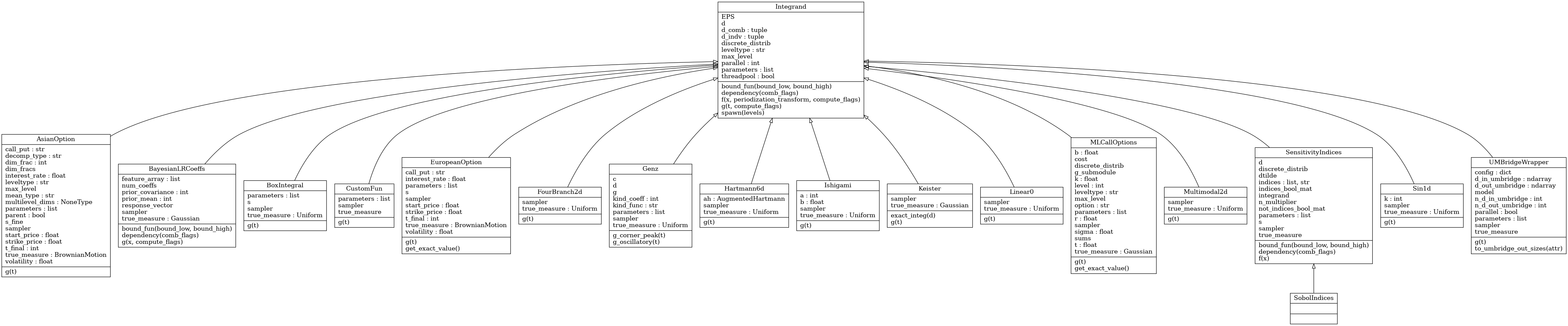
class qmcpy.integrand._integrand.Integrand(dimension_indv, dimension_comb, parallel, threadpool=False)

Integrand abstract class. DO NOT INSTANTIATE.

__init__(dimension_indv, dimension_comb, parallel, threadpool=False)

Parameters

dimension_indv (tuple) – individual solution shape.
dimension_comb (tuple) – combined solution shape.
parallel (int) – If parallel is False, 0, or 1: function evaluation is done in serial fashion. Otherwise, parallel specifies the number of processes used by multiprocessing.Pool or multiprocessing.pool.ThreadPool. Passing parallel=True sets processes = os.cpu_count().
threadpool (bool) – When parallel > 1, if threadpool = True then use multiprocessing.pool.ThreadPool else use multiprocessing.Pool.

bound_fun(bound_low, bound_high)

Compute the bounds on the combined function based on bounds for the individual functions. Defaults to the identity where we essentially do not combine integrands, but instead integrate each function individually.

Parameters

bound_low (ndarray) – length Integrand.d_indv lower error bound
bound_high (ndarray) – length Integrand.d_indv upper error bound

Returns

(tuple) containing

(ndarray): lower bound on function combining estimates
(ndarray): upper bound on function combining estimates
(ndarray): bool flags to override sufficient combined integrand estimation, e.g., when approximating a ratio of integrals, if the denominator’s bounds straddle 0, then returning True here forces ratio to be flagged as insufficiently approximated.

dependency(comb_flags)

Takes a vector of indicators of weather of not the error bound is satisfied for combined integrands and which returns flags for individual integrands. For example, if we are taking the ratio of 2 individual integrands, then getting flag_comb=True means the ratio has not been approximated to within the tolerance, so the dependency function should return [True,True] indicating that both the numerator and denominator integrands need to be better approximated. :param comb_flags: flags indicating weather the combined integrals are insufficiently approximated :type comb_flags: bool ndarray

Returns: length (Integrand.d_indv) flags for individual integrands
Return type: (bool ndarray)

f(x, periodization_transform='NONE', compute_flags=None, *args, **kwargs)

Evaluate transformed integrand based on true measures and discrete distribution

Parameters

x (ndarray) – n x d array of samples from a discrete distribution
periodization_transform (str) – periodization transform
compute_flags (ndarray) – outputs that require computation. For example, if the vector function has 3 outputs and compute_flags = [False, True, False], then the function is only required to compute the second output and may leave the remaining outputs as e.g. 0. The False outputs will not be used in the computation since those integrals have been sufficiently approximated.
*args – other ordered args to g
**kwargs (dict) – other keyword args to g

Returns

length n vector of function evaluations

Return type

ndarray

g(t, compute_flags=None, *args, **kwargs)

ABSTRACT METHOD for original integrand to be integrated.

Parameters

t (ndarray) – n x d array of samples to be input into original integrand.
compute_flags (ndarray) – outputs that require computation. For example, if the vector function has 3 outputs and compute_flags = [False, True, False], then the function is only required to compute the second output and may leave the remaining outputs as e.g. 0. The False outputs will not be used in the computation since those integrals have been sufficiently approximated.

Returns

n vector of function evaluations

Return type

ndarray

spawn(levels)

Spawn new instances of the current integrand at the specified levels.

Parameters: levels (ndarray) – array of levels at which to spawn new integrands
Returns: list of Integrands linked to newly spawned TrueMeasures and DiscreteDistributions
Return type: list

Custom Function

class qmcpy.integrand.custom_fun.CustomFun(true_measure, g, dimension_indv=1, parallel=False)

Integrand wrapper for a user’s function

>>> cf = CustomFun(
...     true_measure = Gaussian(DigitalNetB2(2,seed=7),mean=[1,2]),
...     g = lambda x: x[:,0]**2*x[:,1],
...     dimension_indv = 1)
>>> x = cf.discrete_distrib.gen_samples(2**10)
>>> y = cf.f(x)
>>> y.shape
(1024, 1)
>>> y.mean()
3.995...
>>> cf = CustomFun(
...     true_measure = Uniform(DigitalNetB2(3,seed=7),lower_bound=[2,3,4],upper_bound=[4,5,6]),
...     g = lambda x,compute_flags=None: x,
...     dimension_indv = 3)
>>> x = cf.discrete_distrib.gen_samples(2**10)
>>> y = cf.f(x)
>>> y.shape
(1024, 3)
>>> y.mean(0)
array([3., 4., 5.])

__init__(true_measure, g, dimension_indv=1, parallel=False)

Parameters

true_measure (TrueMeasure) – a TrueMeasure instance.
g (function) – a function handle.
dimension_indv (tuple) – individual solution dimensions.
parallel (int) – If parallel is False, 0, or 1: function evaluation is done in serial fashion. Otherwise, parallel specifies the number of CPUs used by multiprocessing.Pool. Passing parallel=True sets the number of CPUs equal to os.cpu_count(). Do NOT set g to a lambda function when doing parallel computation

g(t, *args, **kwargs)

ABSTRACT METHOD for original integrand to be integrated.

Parameters

t (ndarray) – n x d array of samples to be input into original integrand.
compute_flags (ndarray) – outputs that require computation. For example, if the vector function has 3 outputs and compute_flags = [False, True, False], then the function is only required to compute the second output and may leave the remaining outputs as e.g. 0. The False outputs will not be used in the computation since those integrals have been sufficiently approximated.

Returns

n vector of function evaluations

Return type

ndarray

Keister Function

class qmcpy.integrand.keister.Keister(sampler)

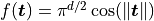$f(\boldsymbol{t}) = \pi^{d/2} \cos(\| \boldsymbol{t} \|)$ .

The standard example integrates the Keister integrand with respect to an IID Gaussian distribution with variance 1./2.

>>> k = Keister(DigitalNetB2(2,seed=7))
>>> x = k.discrete_distrib.gen_samples(2**10)
>>> y = k.f(x)
>>> y.mean()
1.808...
>>> k.true_measure
Gaussian (TrueMeasure Object)
    mean            0
    covariance      2^(-1)
    decomp_type     PCA
>>> k = Keister(Gaussian(DigitalNetB2(2,seed=7),mean=0,covariance=2))
>>> x = k.discrete_distrib.gen_samples(2**12)
>>> y = k.f(x)
>>> y.mean()
1.808...
>>> yp = k.f(x,periodization_transform='c2sin')
>>> yp.mean()
1.807...

References

[1] B. D. Keister, Multidimensional Quadrature Algorithms, Computers in Physics, 10, pp. 119-122, 1996.

__init__(sampler)

Parameters: sampler (DiscreteDistribution/TrueMeasure) – A discrete distribution from which to transform samples or a true measure by which to compose a transform

exact_integ(d): computes the true value of the Keister integral in dimension d. Accuracy might degrade as d increases due to round-off error. :param d: :return: true_integral

g(t)

ABSTRACT METHOD for original integrand to be integrated.

Parameters

t (ndarray) – n x d array of samples to be input into original integrand.
compute_flags (ndarray) – outputs that require computation. For example, if the vector function has 3 outputs and compute_flags = [False, True, False], then the function is only required to compute the second output and may leave the remaining outputs as e.g. 0. The False outputs will not be used in the computation since those integrals have been sufficiently approximated.

Returns

n vector of function evaluations

Return type

ndarray

Box Integral

class qmcpy.integrand.box_integral.BoxIntegral(sampler, s=array([1, 2]))

$B_s(x) = \left(\sum_{j=1}^d x_j^2 \right)^{s/2}$

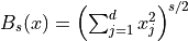
>>> l1 = BoxIntegral(DigitalNetB2(2,seed=7), s=[7])
>>> x1 = l1.discrete_distrib.gen_samples(2**10)
>>> y1 = l1.f(x1)
>>> y1.shape
(1024, 1)
>>> y1.mean(0)
array([0.75156724])
>>> l2 = BoxIntegral(DigitalNetB2(5,seed=7), s=[-7,7])
>>> x2 = l2.discrete_distrib.gen_samples(2**10)
>>> y2 = l2.f(x2,compute_flags=[1,1])
>>> y2.shape
(1024, 2)
>>> y2.mean(0)
array([ 6.67548708, 10.52267786])

References:

[1] D.H. Bailey, J.M. Borwein, R.E. Crandall,Box integrals, Journal of Computational and Applied Mathematics, Volume 206, Issue 1, 2007, Pages 196-208, ISSN 0377-0427, https://doi.org/10.1016/j.cam.2006.06.010. (https://www.sciencedirect.com/science/article/pii/S0377042706004250)

[2] https://www.davidhbailey.com/dhbpapers/boxintegrals.pdf

__init__(sampler, s=array([1, 2]))

Parameters

sampler (DiscreteDistribution/TrueMeasure) – A discrete distribution from which to transform samples or a true measure by which to compose a transform
s (list or ndarray) – vectorized s parameter, len(s) is the number of vectorized integrals to evaluate.

g(t, **kwargs)

ABSTRACT METHOD for original integrand to be integrated.

Parameters

t (ndarray) – n x d array of samples to be input into original integrand.
compute_flags (ndarray) – outputs that require computation. For example, if the vector function has 3 outputs and compute_flags = [False, True, False], then the function is only required to compute the second output and may leave the remaining outputs as e.g. 0. The False outputs will not be used in the computation since those integrals have been sufficiently approximated.

Returns

n vector of function evaluations

Return type

ndarray

European Option

class qmcpy.integrand.european_option.EuropeanOption(sampler, volatility=0.5, start_price=30, strike_price=35, interest_rate=0, t_final=1, call_put='call')

European financial option.

>>> eo = EuropeanOption(DigitalNetB2(4,seed=7),call_put='put')
>>> eo
EuropeanOption (Integrand Object)
    volatility      2^(-1)
    call_put        put
    start_price     30
    strike_price    35
    interest_rate   0
>>> x = eo.discrete_distrib.gen_samples(2**12)
>>> y = eo.f(x)
>>> y.mean()
9.209...
>>> eo = EuropeanOption(BrownianMotion(DigitalNetB2(4,seed=7),drift=1),call_put='put')
>>> x = eo.discrete_distrib.gen_samples(2**12)
>>> y = eo.f(x)
>>> y.mean()
9.162...
>>> eo.get_exact_value()
9.211452976234058

__init__(sampler, volatility=0.5, start_price=30, strike_price=35, interest_rate=0, t_final=1, call_put='call')

Parameters

sampler (DiscreteDistribution/TrueMeasure) – A discrete distribution from which to transform samples or a true measure by which to compose a transform
volatility (float) – sigma, the volatility of the asset
start_price (float) – S(0), the asset value at t=0
strike_price (float) – strike_price, the call/put offer
interest_rate (float) – r, the annual interest rate
t_final (float) – exercise time
call_put (str) – ‘call’ or ‘put’ option

g(t): See abstract method.

get_exact_value()

Get the fair price of a European call/put option.

Returns: fair price
Return type: float

Asian Option

class qmcpy.integrand.asian_option.AsianOption(sampler, volatility=0.5, start_price=30.0, strike_price=35.0, interest_rate=0.0, t_final=1, call_put='call', mean_type='arithmetic', multilevel_dims=None, decomp_type='PCA', _dim_frac=0)

Asian financial option.

>>> ac = AsianOption(DigitalNetB2(4,seed=7))
>>> ac
AsianOption (Integrand Object)
    volatility      2^(-1)
    call_put        call
    start_price     30
    strike_price    35
    interest_rate   0
    mean_type       arithmetic
    dim_frac        0
>>> x = ac.discrete_distrib.gen_samples(2**12)
>>> y = ac.f(x)
>>> y.mean()
1.768...
>>> level_dims = [2,4,8]
>>> ac2_multilevel = AsianOption(DigitalNetB2(seed=7),multilevel_dims=level_dims)
>>> levels_to_spawn = arange(ac2_multilevel.max_level+1)
>>> ac2_single_levels = ac2_multilevel.spawn(levels_to_spawn)
>>> yml = 0
>>> for ac2_single_level in ac2_single_levels:
...     x = ac2_single_level.discrete_distrib.gen_samples(2**12)
...     level_est = ac2_single_level.f(x).mean()
...     yml += level_est
>>> yml
1.779...

__init__(sampler, volatility=0.5, start_price=30.0, strike_price=35.0, interest_rate=0.0, t_final=1, call_put='call', mean_type='arithmetic', multilevel_dims=None, decomp_type='PCA', _dim_frac=0)

Parameters

sampler (DiscreteDistribution/TrueMeasure) – A discrete distribution from which to transform samples or a true measure by which to compose a transform
volatility (float) – sigma, the volatility of the asset
start_price (float) – S(0), the asset value at t=0
strike_price (float) – strike_price, the call/put offer
interest_rate (float) – r, the annual interest rate
t_final (float) – exercise time
mean_type (string) – ‘arithmetic’ or ‘geometric’ mean
multilevel_dims (list of ints) – list of dimensions at each level. Leave as None for single-level problems
_dim_frac (float) – for internal use only, users should not set this parameter.

g(t)

ABSTRACT METHOD for original integrand to be integrated.

Parameters

t (ndarray) – n x d array of samples to be input into original integrand.
compute_flags (ndarray) – outputs that require computation. For example, if the vector function has 3 outputs and compute_flags = [False, True, False], then the function is only required to compute the second output and may leave the remaining outputs as e.g. 0. The False outputs will not be used in the computation since those integrals have been sufficiently approximated.

Returns

n vector of function evaluations

Return type

ndarray

Multilevel Call Options with Milstein Discretization

class qmcpy.integrand.ml_call_options.MLCallOptions(sampler, option='european', volatility=0.2, start_strike_price=100.0, interest_rate=0.05, t_final=1.0, _level=0)

Various call options from finance using Milstein discretization with $2^l$ timesteps on level $l$ .

>>> mlco_original = MLCallOptions(DigitalNetB2(seed=7))
>>> mlco_original
MLCallOptions (Integrand Object)
    option          european
    sigma           0.200
    k               100
    r               0.050
    t               1
    b               85
    level           0
>>> mlco_ml_dims = mlco_original.spawn(levels=arange(4))
>>> yml = 0
>>> for mlco in mlco_ml_dims:
...     x = mlco.discrete_distrib.gen_samples(2**10)
...     yml += mlco.f(x).mean()
>>> yml
10.393...

References:

[1] M.B. Giles. Improved multilevel Monte Carlo convergence using the Milstein scheme. 343-358, in Monte Carlo and Quasi-Monte Carlo Methods 2006, Springer, 2008. http://people.maths.ox.ac.uk/~gilesm/files/mcqmc06.pdf.

__init__(sampler, option='european', volatility=0.2, start_strike_price=100.0, interest_rate=0.05, t_final=1.0, _level=0)

Parameters

sampler (DiscreteDistribution/TrueMeasure) – A discrete distribution from which to transform samples or a true measure by which to compose a transform
option_type (str) – type of option in [“European”,”Asian”]
volatility (float) – sigma, the volatility of the asset
start_strike_price (float) – S(0), the asset value at t=0, and K, the strike price. Assume start_price = strike_price
interest_rate (float) – r, the annual interest rate
t_final (float) – exercise time
_level (int) – for internal use only, users should not set this parameter.

g(t)

Parameters: t (ndarray) – Gaussian(0,1^2) samples
Returns: First, an ndarray of length 6 vector of summary statistic sums. Second, a float of cost on this level.
Return type: tuple

get_exact_value(): Print exact analytic value, based on s0=k.

Linear Function

class qmcpy.integrand.linear0.Linear0(sampler)

>>> l = Linear0(DigitalNetB2(100,seed=7))
>>> x = l.discrete_distrib.gen_samples(2**10)
>>> y = l.f(x)
>>> y.mean()
-1.175...e-08
>>> ytf = l.f(x,periodization_transform='C1SIN')
>>> ytf.mean()
-4.050...e-12

__init__(sampler)

Parameters: sampler (DiscreteDistribution/TrueMeasure) – A discrete distribution from which to transform samples or a true measure by which to compose a transform

g(t)

ABSTRACT METHOD for original integrand to be integrated.

Parameters

t (ndarray) – n x d array of samples to be input into original integrand.
compute_flags (ndarray) – outputs that require computation. For example, if the vector function has 3 outputs and compute_flags = [False, True, False], then the function is only required to compute the second output and may leave the remaining outputs as e.g. 0. The False outputs will not be used in the computation since those integrals have been sufficiently approximated.

Returns

n vector of function evaluations

Return type

ndarray

Bayesian Logistic Regression

class qmcpy.integrand.bayesian_lr_coeffs.BayesianLRCoeffs(sampler, feature_array, response_vector, prior_mean=0, prior_covariance=10)

Logistic Regression Coefficients computed as the posterior mean in a Bayesian framework.

>>> blrcoeffs = BayesianLRCoeffs(DigitalNetB2(3,seed=7),feature_array=arange(8).reshape((4,2)),response_vector=[0,0,1,1])
>>> x = blrcoeffs.discrete_distrib.gen_samples(2**10)
>>> y = blrcoeffs.f(x)
>>> y.shape
(1024, 2, 3)
>>> y.mean(0)
array([[ 0.04639394, -0.01440543, -0.05498496],
       [ 0.02176581,  0.02176581,  0.02176581]])

__init__(sampler, feature_array, response_vector, prior_mean=0, prior_covariance=10)

Parameters

sampler (DiscreteDistribution/TrueMeasure) – A discrete distribution from which to transform samples or a true measure by which to compose a transform
feature_array (ndarray) – N samples by d-1 dimensions array of input features
response_vector (ndarray) – length N array of binary responses corresponding to each
prior_mean (ndarray) – length d array of prior means, one for each coefficient. The first d-1 inputs correspond to the d-1 features. The last input corresponds to the intercept coefficient.
prior_covariance (ndarray) – d x d prior covariance array whose indexing is consistent with the prior mean.

bound_fun(bound_low, bound_high)

Compute the bounds on the combined function based on bounds for the individual functions. Defaults to the identity where we essentially do not combine integrands, but instead integrate each function individually.

Parameters

bound_low (ndarray) – length Integrand.d_indv lower error bound
bound_high (ndarray) – length Integrand.d_indv upper error bound

Returns

(tuple) containing

(ndarray): lower bound on function combining estimates
(ndarray): upper bound on function combining estimates
(ndarray): bool flags to override sufficient combined integrand estimation, e.g., when approximating a ratio of integrals, if the denominator’s bounds straddle 0, then returning True here forces ratio to be flagged as insufficiently approximated.

dependency(comb_flags)

Takes a vector of indicators of weather of not the error bound is satisfied for combined integrands and which returns flags for individual integrands. For example, if we are taking the ratio of 2 individual integrands, then getting flag_comb=True means the ratio has not been approximated to within the tolerance, so the dependency function should return [True,True] indicating that both the numerator and denominator integrands need to be better approximated. :param comb_flags: flags indicating weather the combined integrals are insufficiently approximated :type comb_flags: bool ndarray

Returns: length (Integrand.d_indv) flags for individual integrands
Return type: (bool ndarray)

g(x, compute_flags)

ABSTRACT METHOD for original integrand to be integrated.

Parameters

t (ndarray) – n x d array of samples to be input into original integrand.
compute_flags (ndarray) – outputs that require computation. For example, if the vector function has 3 outputs and compute_flags = [False, True, False], then the function is only required to compute the second output and may leave the remaining outputs as e.g. 0. The False outputs will not be used in the computation since those integrals have been sufficiently approximated.

Returns

n vector of function evaluations

Return type

ndarray

Genz Function

class qmcpy.integrand.genz.Genz(sampler, kind_func='oscilatory', kind_coeff=1)

https://dakota.sandia.gov/sites/default/files/docs/6.17.0-release/user-html/usingdakota/examples/additionalexamples.html?highlight=genz#genz-functions

>>> for kind_func in ['oscilatory','corner-peak']:
...     for kind_coeff in [1,2,3]:
...         g = Genz(DigitalNetB2(2,seed=7),kind_func=kind_func,kind_coeff=kind_coeff)
...         x = g.discrete_distrib.gen_samples(2**14)
...         y = g.f(x)
...         mu_hat = y.mean()
...         print('%-15s %-3d %.3f'%(kind_func,kind_coeff,mu_hat))
oscilatory      1   -0.351
oscilatory      2   -0.380
oscilatory      3   -0.217
corner-peak     1   0.713
corner-peak     2   0.712
corner-peak     3   0.720

__init__(sampler, kind_func='oscilatory', kind_coeff=1)

Parameters

sampler (DiscreteDistribution/TrueMeasure) – A discrete distribution from which to transform samples or a true measure by which to compose a transform
kind_func (str) – ‘oscilatory’ or ‘corner-peak’
kind_coeff (int) – 1, 2, or 3 for choice of coefficients

Ishigami Function

class qmcpy.integrand.ishigami.Ishigami(sampler, a=7, b=0.1)

$g(\boldsymbol{t}) = (1+bt_2^4)\sin(t_0) + a\sin^2(t_1), \qquad T \sim \mathcal{U}(-\pi,\pi)^3$

https://www.sfu.ca/~ssurjano/ishigami.html

>>> ishigami = Ishigami(DigitalNetB2(3,seed=7))
>>> x = ishigami.discrete_distrib.gen_samples(2**10)
>>> y = ishigami.f(x)
>>> y.mean()
3.499...
>>> ishigami.true_measure
Uniform (TrueMeasure Object)
    lower_bound     -3.142
    upper_bound     3.142

References: [1] Ishigami, T., & Homma, T. (1990, December). An importance quantification technique in uncertainty analysis for computer models. In Uncertainty Modeling and Analysis, 1990. Proceedings., First International Symposium on (pp. 398-403). IEEE.

__init__(sampler, a=7, b=0.1)

Parameters

sampler (DiscreteDistribution/TrueMeasure) – A discrete distribution from which to transform samples or a true measure by which to compose a transform
a (float) – fixed parameters in above equation
b (float) – fixed parameters in above equation

g(t)

ABSTRACT METHOD for original integrand to be integrated.

Parameters

t (ndarray) – n x d array of samples to be input into original integrand.
compute_flags (ndarray) – outputs that require computation. For example, if the vector function has 3 outputs and compute_flags = [False, True, False], then the function is only required to compute the second output and may leave the remaining outputs as e.g. 0. The False outputs will not be used in the computation since those integrals have been sufficiently approximated.

Returns

n vector of function evaluations

Return type

ndarray

Sensitivity Indices

class qmcpy.integrand.sensitivity_indices.SensitivityIndices(integrand, indices='singletons')

Sensitivity’ Indicies, normalized Sobol’ Indices.

>>> dnb2 = DigitalNetB2(dimension=3,seed=7)
>>> keister_d = Keister(dnb2)
>>> keister_indices = SensitivityIndices(keister_d,indices='singletons')
>>> sc = CubQMCNetG(keister_indices,abs_tol=1e-3)
>>> solution,data = sc.integrate()
>>> solution.squeeze()
array([[0.32803639, 0.32795358, 0.32807359],
       [0.33884667, 0.33857811, 0.33884115]])
>>> data
LDTransformData (AccumulateData Object)
    solution        [[0.328 0.328 0.328]
                    [0.339 0.339 0.339]]
    comb_bound_low  [[0.327 0.327 0.328]
                    [0.338 0.338 0.338]]
    comb_bound_high [[0.329 0.329 0.329]
                    [0.34  0.339 0.34 ]]
    comb_flags      [[ True  True  True]
                    [ True  True  True]]
    n_total         2^(16)
    n               [[[65536. 65536. 65536.]
                     [65536. 65536. 65536.]
                     [65536. 65536. 65536.]]

                    [[32768. 32768. 32768.]
                     [32768. 32768. 32768.]
                     [32768. 32768. 32768.]]]
    time_integrate  ...
CubQMCNetG (StoppingCriterion Object)
    abs_tol         0.001
    rel_tol         0
    n_init          2^(10)
    n_max           2^(35)
SensitivityIndices (Integrand Object)
    indices         [[0]
                    [1]
                    [2]]
    n_multiplier    3
Gaussian (TrueMeasure Object)
    mean            0
    covariance      2^(-1)
    decomp_type     PCA
DigitalNetB2 (DiscreteDistribution Object)
    d               6
    dvec            [0 1 2 3 4 5]
    randomize       LMS_DS
    graycode        0
    entropy         7
    spawn_key       (0,)
>>> sc = CubQMCNetG(SobolIndices(BoxIntegral(DigitalNetB2(3,seed=7)),indices='all'),abs_tol=.01)
>>> sol,data = sc.integrate()
>>> print(sol)
[[[0.32312991 0.33340559]
  [0.32331463 0.33342669]
  [0.32160276 0.33318619]
  [0.65559598 0.6667154 ]
  [0.65551702 0.66670251]
  [0.6556618  0.66672429]]

 [[0.3440018  0.33341845]
  [0.34501082 0.33347005]
  [0.34504829 0.33345212]
  [0.67659368 0.6667021 ]
  [0.67725088 0.66667925]
  [0.67802866 0.66672587]]]

References

[1] Art B. Owen.Monte Carlo theory, methods and examples. 2013. Appendix A.

__init__(integrand, indices='singletons')

Parameters

integrand (Integrand) – integrand to find Sobol’ indices of
indices (list of lists) – each element of indices should be a list of indices, u, at which to compute the Sobol’ indices. The default indices=’singletons’ sets indices=[[0],[1],…[d-1]]. Should not include [], the null set, or [0,…,d-1], the set of all indices. Setting indices=’all’ will compute all sensitivity indices

bound_fun(bound_low, bound_high)

Compute the bounds on the combined function based on bounds for the individual functions. Defaults to the identity where we essentially do not combine integrands, but instead integrate each function individually.

Parameters

bound_low (ndarray) – length Integrand.d_indv lower error bound
bound_high (ndarray) – length Integrand.d_indv upper error bound

Returns

(tuple) containing

(ndarray): lower bound on function combining estimates
(ndarray): upper bound on function combining estimates
(ndarray): bool flags to override sufficient combined integrand estimation, e.g., when approximating a ratio of integrals, if the denominator’s bounds straddle 0, then returning True here forces ratio to be flagged as insufficiently approximated.

dependency(comb_flags)

Takes a vector of indicators of weather of not the error bound is satisfied for combined integrands and which returns flags for individual integrands. For example, if we are taking the ratio of 2 individual integrands, then getting flag_comb=True means the ratio has not been approximated to within the tolerance, so the dependency function should return [True,True] indicating that both the numerator and denominator integrands need to be better approximated. :param comb_flags: flags indicating weather the combined integrals are insufficiently approximated :type comb_flags: bool ndarray

Returns: length (Integrand.d_indv) flags for individual integrands
Return type: (bool ndarray)

f(x, *args, **kwargs)

Evaluate transformed integrand based on true measures and discrete distribution

Parameters

x (ndarray) – n x d array of samples from a discrete distribution
periodization_transform (str) – periodization transform
compute_flags (ndarray) – outputs that require computation. For example, if the vector function has 3 outputs and compute_flags = [False, True, False], then the function is only required to compute the second output and may leave the remaining outputs as e.g. 0. The False outputs will not be used in the computation since those integrals have been sufficiently approximated.
*args – other ordered args to g
**kwargs (dict) – other keyword args to g

Returns

length n vector of function evaluations

Return type

ndarray

class qmcpy.integrand.sensitivity_indices.SobolIndices(integrand, indices='singletons'): Normalized Sobol’ Indices, an alias for SensitivityIndices.

UM-Bridge Wrapper

class qmcpy.integrand.um_bridge_wrapper.UMBridgeWrapper(true_measure, model, config={}, parallel=False)

UM-Bridge Model Wrapper. Requires Docker be installed, see https://www.docker.com/.

>>> _ = os.system('docker run --name muqbp -dit -p 4243:4243 linusseelinger/benchmark-muq-beam-propagation:latest > /dev/null')
>>> import umbridge
>>> dnb2 = DigitalNetB2(dimension=3,seed=7)
>>> distribution = Uniform(dnb2,lower_bound=1,upper_bound=1.05)
>>> model = umbridge.HTTPModel('http://localhost:4243','forward')
>>> umbridge_config = {"d": dnb2.d}
>>> um_bridge_integrand = UMBridgeWrapper(distribution,model,umbridge_config,parallel=False)
>>> solution,data = CubQMCNetG(um_bridge_integrand,abs_tol=5e-2).integrate()
>>> print(data)
LDTransformData (AccumulateData Object)
    solution        [  0.      3.855  14.69  ... 898.921 935.383 971.884]
    comb_bound_low  [  0.      3.854  14.688 ... 898.901 935.363 971.863]
    comb_bound_high [  0.      3.855  14.691 ... 898.941 935.404 971.906]
    comb_flags      [ True  True  True ...  True  True  True]
    n_total         2^(11)
    n               [1024. 1024. 1024. ... 2048. 2048. 2048.]
    time_integrate  ...
CubQMCNetG (StoppingCriterion Object)
    abs_tol         0.050
    rel_tol         0
    n_init          2^(10)
    n_max           2^(35)
UMBridgeWrapper (Integrand Object)
Uniform (TrueMeasure Object)
    lower_bound     1
    upper_bound     1.050
DigitalNetB2 (DiscreteDistribution Object)
    d               3
    dvec            [0 1 2]
    randomize       LMS_DS
    graycode        0
    entropy         7
    spawn_key       ()
>>> _ = os.system('docker rm -f muqbp > /dev/null')
>>> class TestModel(umbridge.Model):
...     def __init__(self):
...         super().__init__("forward")
...     def get_input_sizes(self, config):
...         return [1,2,3]
...     def get_output_sizes(self, config):
...         return [3,2,1]
...     def __call__(self, parameters, config):
...         out0 = [parameters[2][0],sum(parameters[2][:2]),sum(parameters[2])]
...         out1 = [parameters[1][0],sum(parameters[1])]
...         out2 = [parameters[0]]
...         return [out0,out1,out2]
...     def supports_evaluate(self):
...         return True
>>> my_model = TestModel()
>>> my_distribution = Uniform(
...     sampler = DigitalNetB2(dimension=sum(my_model.get_input_sizes(config={})),seed=7),
...     lower_bound = -1,
...     upper_bound = 1)
>>> my_integrand = UMBridgeWrapper(my_distribution,my_model)
>>> my_solution,my_data = CubQMCNetG(my_integrand,abs_tol=5e-2).integrate()
>>> my_data
LDTransformData (AccumulateData Object)
    solution        [-2.328e-10 -4.657e-10 -6.985e-10 -2.328e-10 -4.657e-10 -2.328e-10]
    comb_bound_low  [-9.649e-06 -1.765e-04 -2.352e-04 -3.053e-07 -1.997e-05 -1.952e-05]
    comb_bound_high [9.649e-06 1.765e-04 2.352e-04 3.048e-07 1.997e-05 1.952e-05]
    comb_flags      [ True  True  True  True  True  True]
    n_total         2^(10)
    n               [1024. 1024. 1024. 1024. 1024. 1024.]
    time_integrate  ...
CubQMCNetG (StoppingCriterion Object)
    abs_tol         0.050
    rel_tol         0
    n_init          2^(10)
    n_max           2^(35)
UMBridgeWrapper (Integrand Object)
Uniform (TrueMeasure Object)
    lower_bound     -1
    upper_bound     1
DigitalNetB2 (DiscreteDistribution Object)
    d               6
    dvec            [0 1 2 3 4 5]
    randomize       LMS_DS
    graycode        0
    entropy         7
    spawn_key       ()
>>> my_integrand.to_umbridge_out_sizes(my_solution)
[[-2.3283064365386963e-10, -4.656612873077393e-10, -6.984919309616089e-10], [-2.3283064365386963e-10, -4.656612873077393e-10], [-2.3283064365386963e-10]]
>>> my_integrand.to_umbridge_out_sizes(my_data.comb_bound_low)
[[-9.649316780269146e-06, -0.00017654551993473433, -0.00023524149401055183], [-3.0527962735504843e-07, -1.997367189687793e-05], [-1.9521190552040935e-05]]
>>> my_integrand.to_umbridge_out_sizes(my_data.comb_bound_high)
[[9.648851118981838e-06, 0.00017654458861215971, 0.0002352400970266899], [3.048139660677407e-07, 1.9972740574303316e-05], [1.9520724890753627e-05]]

References

[1] UM-Bridge documentation. https://um-bridge-benchmarks.readthedocs.io/en/docs/index.html

__init__(true_measure, model, config={}, parallel=False)

See https://um-bridge-benchmarks.readthedocs.io/en/docs/umbridge/clients.html

Parameters

true_measure (TrueMeasure) – a TrueMeasure instance.
model (umbridge.HTTPModel) – a UM-Bridge model
config (dict) – config keyword argument to umbridge.HTTPModel(url,name).__call__
parallel (int) – If parallel is False, 0, or 1: function evaluation is done in serial fashion. Otherwise, parallel specifies the number of processes used by multiprocessing.Pool or multiprocessing.pool.ThreadPool. Passing parallel=True sets processes = os.cpu_count().

g(t, **kwargs)

ABSTRACT METHOD for original integrand to be integrated.

Parameters

t (ndarray) – n x d array of samples to be input into original integrand.
compute_flags (ndarray) – outputs that require computation. For example, if the vector function has 3 outputs and compute_flags = [False, True, False], then the function is only required to compute the second output and may leave the remaining outputs as e.g. 0. The False outputs will not be used in the computation since those integrals have been sufficiently approximated.

Returns

n vector of function evaluations

Return type

ndarray

to_umbridge_out_sizes(attr)

Convert a data attribute to UM-Bridge output sized list of lists.

Parameters: attr (ndarray) – array of length sum(model.get_output_sizes(self.config))
Returns: list of lists with sub-list lengths specified by model.get_output_sizes(self.config)
Return type: list

Sin 1d

class qmcpy.integrand.sin1d.Sin1d(sampler, k=1)

>>> sin1d = Sin1d(DigitalNetB2(1,seed=7))
>>> x = sin1d.discrete_distrib.gen_samples(2**10)
>>> y = sin1d.f(x)
>>> y.mean()
7.33449186...e-08
>>> sin1d.true_measure
Uniform (TrueMeasure Object)
    lower_bound     0
    upper_bound     6.283

g(t)

ABSTRACT METHOD for original integrand to be integrated.

Parameters

t (ndarray) – n x d array of samples to be input into original integrand.
compute_flags (ndarray) – outputs that require computation. For example, if the vector function has 3 outputs and compute_flags = [False, True, False], then the function is only required to compute the second output and may leave the remaining outputs as e.g. 0. The False outputs will not be used in the computation since those integrals have been sufficiently approximated.

Returns

n vector of function evaluations

Return type

ndarray

Multimodal 2d

class qmcpy.integrand.multimodal2d.Multimodal2d(sampler)

>>> mm2d = Multimodal2d(DigitalNetB2(2,seed=7))
>>> x = mm2d.discrete_distrib.gen_samples(2**10)
>>> y = mm2d.f(x)
>>> y.mean()
-0.7365118306607449
>>> mm2d.true_measure
Uniform (TrueMeasure Object)
    lower_bound     [-4 -3]
    upper_bound     [7 8]

g(t)

ABSTRACT METHOD for original integrand to be integrated.

Parameters

t (ndarray) – n x d array of samples to be input into original integrand.
compute_flags (ndarray) – outputs that require computation. For example, if the vector function has 3 outputs and compute_flags = [False, True, False], then the function is only required to compute the second output and may leave the remaining outputs as e.g. 0. The False outputs will not be used in the computation since those integrals have been sufficiently approximated.

Returns

n vector of function evaluations

Return type

ndarray

Four Branch 2d

class qmcpy.integrand.fourbranch2d.FourBranch2d(sampler)

>>> fb2d = FourBranch2d(DigitalNetB2(2,seed=7))
>>> x = fb2d.discrete_distrib.gen_samples(2**10)
>>> y = fb2d.f(x)
>>> y.mean()
-2.5003746135324247
>>> fb2d.true_measure
Uniform (TrueMeasure Object)
    lower_bound     -8
    upper_bound     2^(3)

g(t)

ABSTRACT METHOD for original integrand to be integrated.

Parameters

t (ndarray) – n x d array of samples to be input into original integrand.
compute_flags (ndarray) – outputs that require computation. For example, if the vector function has 3 outputs and compute_flags = [False, True, False], then the function is only required to compute the second output and may leave the remaining outputs as e.g. 0. The False outputs will not be used in the computation since those integrals have been sufficiently approximated.

Returns

n vector of function evaluations

Return type

ndarray

Hartmann 6d

class qmcpy.integrand.hartmann6d.Hartmann6d(sampler)

>>> h6d = Hartmann6d(DigitalNetB2(6,seed=7))
>>> x = h6d.discrete_distrib.gen_samples(2**10)
>>> y = h6d.f(x)
>>> y.mean()
-0.2613140309713834
>>> h6d.true_measure
Uniform (TrueMeasure Object)
    lower_bound     0
    upper_bound     1

g(t)

ABSTRACT METHOD for original integrand to be integrated.

Parameters

t (ndarray) – n x d array of samples to be input into original integrand.
compute_flags (ndarray) – outputs that require computation. For example, if the vector function has 3 outputs and compute_flags = [False, True, False], then the function is only required to compute the second output and may leave the remaining outputs as e.g. 0. The False outputs will not be used in the computation since those integrals have been sufficiently approximated.

Returns

n vector of function evaluations

Return type

ndarray

Stopping Criterion Algorithms

Abstract Stopping Criterion Class

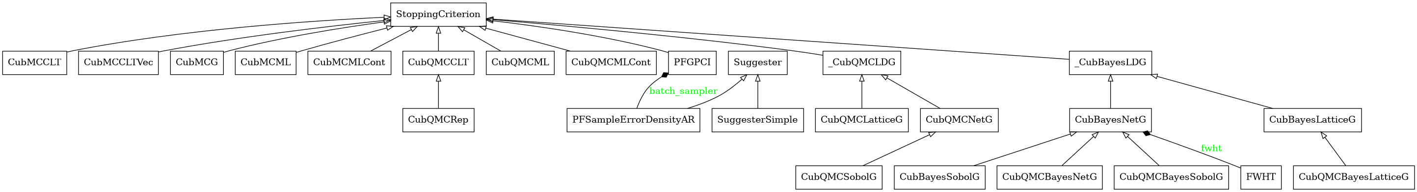
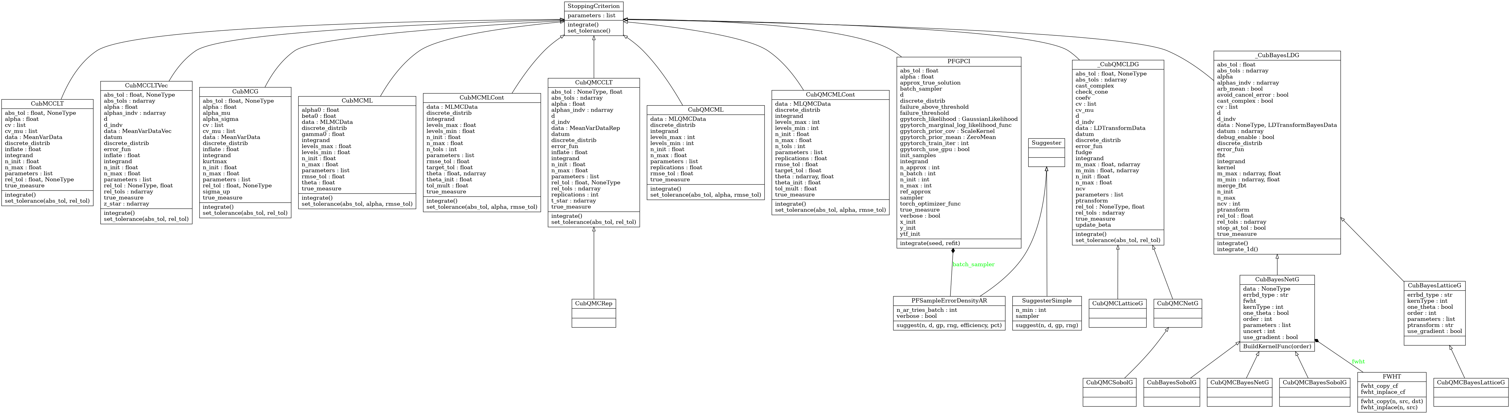
class qmcpy.stopping_criterion._stopping_criterion.StoppingCriterion(allowed_levels, allowed_distribs, allow_vectorized_integrals)

Stopping Criterion abstract class. DO NOT INSTANTIATE.

__init__(allowed_levels, allowed_distribs, allow_vectorized_integrals)

Parameters

distribution (DiscreteDistribution) – a DiscreteDistribution
allowed_levels (list) – which integrand types are supported: ‘single’, ‘fixed-multi’, ‘adaptive-multi’
allowed_distribs (list) – list of compatible DiscreteDistribution classes

integrate()

ABSTRACT METHOD to determine the number of samples needed to satisfy the tolerance.

Returns

tuple containing:

solution (float): approximation to the integral
data (AccumulateData): an AccumulateData object

Return type

tuple

set_tolerance(*args, **kwargs): ABSTRACT METHOD to reset the absolute tolerance.

Guaranteed Digital Net Cubature (QMC)

class qmcpy.stopping_criterion.cub_qmc_net_g.CubQMCNetG(integrand, abs_tol=0.01, rel_tol=0.0, n_init=1024.0, n_max=34359738368.0, fudge=<function CubQMCNetG.<lambda>>, check_cone=False, control_variates=[], control_variate_means=[], update_beta=False, error_fun=<function CubQMCNetG.<lambda>>)

Quasi-Monte Carlo method using Sobol’ cubature over the d-dimensional region to integrate within a specified generalized error tolerance with guarantees under Walsh-Fourier coefficients cone decay assumptions.

>>> k = Keister(DigitalNetB2(2,seed=7))
>>> sc = CubQMCNetG(k,abs_tol=.05)
>>> solution,data = sc.integrate()
>>> data
LDTransformData (AccumulateData Object)
    solution        1.809
    comb_bound_low  1.804
    comb_bound_high 1.814
    comb_flags      1
    n_total         2^(10)
    n               2^(10)
    time_integrate  ...
CubQMCNetG (StoppingCriterion Object)
    abs_tol         0.050
    rel_tol         0
    n_init          2^(10)
    n_max           2^(35)
Keister (Integrand Object)
Gaussian (TrueMeasure Object)
    mean            0
    covariance      2^(-1)
    decomp_type     PCA
DigitalNetB2 (DiscreteDistribution Object)
    d               2^(1)
    dvec            [0 1]
    randomize       LMS_DS
    graycode        0
    entropy         7
    spawn_key       ()
>>> dd = DigitalNetB2(3,seed=7)
>>> g1 = CustomFun(Uniform(dd,0,2),lambda t: 10*t[:,0]-5*t[:,1]**2+t[:,2]**3)
>>> cv1 = CustomFun(Uniform(dd,0,2),lambda t: t[:,0])
>>> cv2 = CustomFun(Uniform(dd,0,2),lambda t: t[:,1]**2)
>>> sc = CubQMCNetG(g1,abs_tol=1e-6,check_cone=True,
...     control_variates = [cv1,cv2],
...     control_variate_means = [1,4/3])
>>> sol,data = sc.integrate()
>>> sol
array([5.33333333])
>>> exactsol = 16/3
>>> abs(sol-exactsol)<1e-6
array([ True])
>>> dnb2 = DigitalNetB2(3,seed=7)
>>> f = BoxIntegral(dnb2, s=[-1,1])
>>> abs_tol = 1e-3
>>> sc = CubQMCNetG(f, abs_tol=abs_tol)
>>> solution,data = sc.integrate()
>>> solution
array([1.18944142, 0.96064165])
>>> sol3neg1 = -pi/4-1/2*log(2)+log(5+3*sqrt(3))
>>> sol31 = sqrt(3)/4+1/2*log(2+sqrt(3))-pi/24
>>> true_value = array([sol3neg1,sol31])
>>> (abs(true_value-solution)<abs_tol).all()
True
>>> f2 = BoxIntegral(dnb2,s=[3,4])
>>> sc = CubQMCNetG(f2,control_variates=f,control_variate_means=true_value,update_beta=True)
>>> solution,data = sc.integrate()
>>> solution
array([1.10168119, 1.26661293])
>>> data
LDTransformData (AccumulateData Object)
    solution        [1.102 1.267]
    comb_bound_low  [1.099 1.262]
    comb_bound_high [1.104 1.271]
    comb_flags      [ True  True]
    n_total         2^(10)
    n               [1024. 1024.]
    time_integrate  ...
CubQMCNetG (StoppingCriterion Object)
    abs_tol         0.010
    rel_tol         0
    n_init          2^(10)
    n_max           2^(35)
    cv              BoxIntegral (Integrand Object)
                       s               [-1  1]
    cv_mu           [1.19  0.961]
    update_beta     1
BoxIntegral (Integrand Object)
    s               [3 4]
Uniform (TrueMeasure Object)
    lower_bound     0
    upper_bound     1
DigitalNetB2 (DiscreteDistribution Object)
    d               3
    dvec            [0 1 2]
    randomize       LMS_DS
    graycode        0
    entropy         7
    spawn_key       ()
>>> cf = CustomFun(
...     true_measure = Uniform(DigitalNetB2(6,seed=7)),
...     g = lambda x,compute_flags=None: (2*arange(1,7)*x).reshape(-1,2,3),
...     dimension_indv = (2,3))
>>> sol,data = CubQMCNetG(cf,abs_tol=1e-6).integrate()
>>> data
LDTransformData (AccumulateData Object)
    solution        [[1. 2. 3.]
                    [4. 5. 6.]]
    comb_bound_low  [[1. 2. 3.]
                    [4. 5. 6.]]
    comb_bound_high [[1. 2. 3.]
                    [4. 5. 6.]]
    comb_flags      [[ True  True  True]
                    [ True  True  True]]
    n_total         2^(13)
    n               [[2048. 1024. 1024.]
                    [8192. 4096. 2048.]]
    time_integrate  ...
CubQMCNetG (StoppingCriterion Object)
    abs_tol         1.00e-06
    rel_tol         0
    n_init          2^(10)
    n_max           2^(35)
CustomFun (Integrand Object)
Uniform (TrueMeasure Object)
    lower_bound     0
    upper_bound     1
DigitalNetB2 (DiscreteDistribution Object)
    d               6
    dvec            [0 1 2 3 4 5]
    randomize       LMS_DS
    graycode        0
    entropy         7
    spawn_key       ()

Original Implementation:

https://github.com/GailGithub/GAIL_Dev/blob/master/Algorithms/IntegrationExpectation/cubSobol_g.m

References

[1] Fred J. Hickernell and Lluis Antoni Jimenez Rugama, Reliable adaptive cubature using digital sequences, 2014. Submitted for publication: arXiv:1410.8615.

[2] Sou-Cheng T. Choi, Yuhan Ding, Fred J. Hickernell, Lan Jiang, Lluis Antoni Jimenez Rugama, Da Li, Jagadeeswaran Rathinavel, Xin Tong, Kan Zhang, Yizhi Zhang, and Xuan Zhou, GAIL: Guaranteed Automatic Integration Library (Version 2.3) [MATLAB Software], 2019. Available from http://gailgithub.github.io/GAIL_Dev/

Guarantee:: This algorithm computes the integral of real valued functions in $[0,1]^d$ with a prescribed generalized error tolerance. The Fourier coefficients of the integrand are assumed to be absolutely convergent. If the algorithm terminates without warning messages, the output is given with guarantees under the assumption that the integrand lies inside a cone of functions. The guarantee is based on the decay rate of the Fourier coefficients. For integration over domains other than $[0,1]^d$ , this cone condition applies to $f \circ \psi$ (the composition of the functions) where $\psi$ is the transformation function for $[0,1]^d$ to the desired region. For more details on how the cone is defined, please refer to the references below.

__init__(integrand, abs_tol=0.01, rel_tol=0.0, n_init=1024.0, n_max=34359738368.0, fudge=<function CubQMCNetG.<lambda>>, check_cone=False, control_variates=[], control_variate_means=[], update_beta=False, error_fun=<function CubQMCNetG.<lambda>>)

Parameters

integrand (Integrand) – an instance of Integrand
abs_tol (ndarray) – absolute error tolerance
rel_tol (ndarray) – relative error tolerance
n_init (int) – initial number of samples
n_max (int) – maximum number of samples
fudge (function) – positive function multiplying the finite sum of Fast Fourier coefficients specified in the cone of functions
check_cone (boolean) – check if the function falls in the cone
control_variates (list) – list of integrand objects to be used as control variates. Control variates are currently only compatible with single level problems. The same discrete distribution instance must be used for the integrand and each of the control variates.
control_variate_means (list) – list of means for each control variate
update_beta (bool) – update control variate beta coefficients at each iteration
error_fun – function taking in the approximate solution vector, absolute tolerance, and relative tolerance which returns the approximate error. Default indicates integration until either absolute OR relative tolerance is satisfied.

class qmcpy.stopping_criterion.cub_qmc_net_g.CubQMCSobolG(integrand, abs_tol=0.01, rel_tol=0.0, n_init=1024.0, n_max=34359738368.0, fudge=<function CubQMCNetG.<lambda>>, check_cone=False, control_variates=[], control_variate_means=[], update_beta=False, error_fun=<function CubQMCNetG.<lambda>>)

Guaranteed Lattice Cubature (QMC)

class qmcpy.stopping_criterion.cub_qmc_lattice_g.CubQMCLatticeG(integrand, abs_tol=0.01, rel_tol=0.0, n_init=1024.0, n_max=34359738368.0, fudge=<function CubQMCLatticeG.<lambda>>, check_cone=False, ptransform='Baker', error_fun=<function CubQMCLatticeG.<lambda>>)

Stopping Criterion quasi-Monte Carlo method using rank-1 Lattices cubature over a d-dimensional region to integrate within a specified generalized error tolerance with guarantees under Fourier coefficients cone decay assumptions.

>>> k = Keister(Lattice(2,seed=7))
>>> sc = CubQMCLatticeG(k,abs_tol=.05)
>>> solution,data = sc.integrate()
>>> data
LDTransformData (AccumulateData Object)
    solution        1.810
    comb_bound_low  1.806
    comb_bound_high 1.815
    comb_flags      1
    n_total         2^(10)
    n               2^(10)
    time_integrate  ...
CubQMCLatticeG (StoppingCriterion Object)
    abs_tol         0.050
    rel_tol         0
    n_init          2^(10)
    n_max           2^(35)
Keister (Integrand Object)
Gaussian (TrueMeasure Object)
    mean            0
    covariance      2^(-1)
    decomp_type     PCA
Lattice (DiscreteDistribution Object)
    d               2^(1)
    dvec            [0 1]
    randomize       1
    order           natural
    gen_vec         [     1 182667]
    entropy         7
    spawn_key       ()
>>> f = BoxIntegral(Lattice(3,seed=7), s=[-1,1])
>>> abs_tol = 1e-3
>>> sc = CubQMCLatticeG(f, abs_tol=abs_tol)
>>> solution,data = sc.integrate()
>>> solution
array([1.18954582, 0.96056304])
>>> sol3neg1 = -pi/4-1/2*log(2)+log(5+3*sqrt(3))
>>> sol31 = sqrt(3)/4+1/2*log(2+sqrt(3))-pi/24
>>> true_value = array([sol3neg1,sol31])
>>> (abs(true_value-solution)<abs_tol).all()
True
>>> cf = CustomFun(
...     true_measure = Uniform(Lattice(6,seed=7)),
...     g = lambda x,compute_flags=None: (2*arange(1,7)*x).reshape(-1,2,3),
...     dimension_indv = (2,3))
>>> sol,data = CubQMCLatticeG(cf,abs_tol=1e-6).integrate()
>>> data
LDTransformData (AccumulateData Object)
    solution        [[1. 2. 3.]
                    [4. 5. 6.]]
    comb_bound_low  [[1. 2. 3.]
                    [4. 5. 6.]]
    comb_bound_high [[1. 2. 3.]
                    [4. 5. 6.]]
    comb_flags      [[ True  True  True]
                    [ True  True  True]]
    n_total         2^(15)
    n               [[ 8192. 16384. 16384.]
                    [16384. 32768. 32768.]]
    time_integrate  ...
CubQMCLatticeG (StoppingCriterion Object)
    abs_tol         1.00e-06
    rel_tol         0
    n_init          2^(10)
    n_max           2^(35)
CustomFun (Integrand Object)
Uniform (TrueMeasure Object)
    lower_bound     0
    upper_bound     1
Lattice (DiscreteDistribution Object)
    d               6
    dvec            [0 1 2 3 4 5]
    randomize       1
    order           natural
    gen_vec         [     1 182667 469891 498753 110745 446247]
    entropy         7
    spawn_key       ()

Original Implementation:

https://github.com/GailGithub/GAIL_Dev/blob/master/Algorithms/IntegrationExpectation/cubLattice_g.m

References

[1] Lluis Antoni Jimenez Rugama and Fred J. Hickernell, “Adaptive multidimensional integration based on rank-1 lattices,” Monte Carlo and Quasi-Monte Carlo Methods: MCQMC, Leuven, Belgium, April 2014 (R. Cools and D. Nuyens, eds.), Springer Proceedings in Mathematics and Statistics, vol. 163, Springer-Verlag, Berlin, 2016, arXiv:1411.1966, pp. 407-422.

[2] Sou-Cheng T. Choi, Yuhan Ding, Fred J. Hickernell, Lan Jiang, Lluis Antoni Jimenez Rugama, Da Li, Jagadeeswaran Rathinavel, Xin Tong, Kan Zhang, Yizhi Zhang, and Xuan Zhou, GAIL: Guaranteed Automatic Integration Library (Version 2.3) [MATLAB Software], 2019. Available from http://gailgithub.github.io/GAIL_Dev/

Guarantee:: This algorithm computes the integral of real valued functions in $[0,1]^d$ with a prescribed generalized error tolerance. The Fourier coefficients of the integrand are assumed to be absolutely convergent. If the algorithm terminates without warning messages, the output is given with guarantees under the assumption that the integrand lies inside a cone of functions. The guarantee is based on the decay rate of the Fourier coefficients. For integration over domains other than $[0,1]^d$ , this cone condition applies to $f \circ \psi$ (the composition of the functions) where $\psi$ is the transformation function for $[0,1]^d$ to the desired region. For more details on how the cone is defined, please refer to the references below.

__init__(integrand, abs_tol=0.01, rel_tol=0.0, n_init=1024.0, n_max=34359738368.0, fudge=<function CubQMCLatticeG.<lambda>>, check_cone=False, ptransform='Baker', error_fun=<function CubQMCLatticeG.<lambda>>)

Parameters

integrand (Integrand) – an instance of Integrand
abs_tol (ndarray) – absolute error tolerance
rel_tol (ndarray) – relative error tolerance
n_init (int) – initial number of samples
n_max (int) – maximum number of samples
fudge (function) – positive function multiplying the finite sum of Fast Fourier coefficients specified in the cone of functions
check_cone (boolean) – check if the function falls in the cone
error_fun – function taking in the approximate solution vector, absolute tolerance, and relative tolerance which returns the approximate error. Default indicates integration until either absolute OR relative tolerance is satisfied.

Bayesian Lattice Cubature (QMC)

class qmcpy.stopping_criterion.cub_qmc_bayes_lattice_g.CubBayesLatticeG(integrand, abs_tol=0.01, rel_tol=0, n_init=256, n_max=4194304, order=2, alpha=0.01, ptransform='C1sin', error_fun=<function CubBayesLatticeG.<lambda>>)

Stopping criterion for Bayesian Cubature using rank-1 Lattice sequence with guaranteed accuracy over a d-dimensional region to integrate within a specified generalized error tolerance with guarantees under Bayesian assumptions.

>>> k = Keister(Lattice(2, order='linear', seed=123456789))
>>> sc = CubBayesLatticeG(k,abs_tol=.05)
>>> solution,data = sc.integrate()
>>> data
LDTransformBayesData (AccumulateData Object)
    solution        1.808
    comb_bound_low  1.808
    comb_bound_high 1.809
    comb_flags      1
    n_total         2^(8)
    n               2^(8)
    time_integrate  ...
CubBayesLatticeG (StoppingCriterion Object)
    abs_tol         0.050
    rel_tol         0
    n_init          2^(8)
    n_max           2^(22)
    order           2^(1)
Keister (Integrand Object)
Gaussian (TrueMeasure Object)
    mean            0
    covariance      2^(-1)
    decomp_type     PCA
Lattice (DiscreteDistribution Object)
    d               2^(1)
    dvec            [0 1]
    randomize       1
    order           linear
    gen_vec         [     1 182667]
    entropy         123456789
    spawn_key       ()

Adapted from GAIL cubBayesLattice_g.

Guarantees:

This algorithm attempts to calculate the integral of function $f$ over the hyperbox $[0,1]^d$ to a prescribed error tolerance $\mbox{tolfun} := max(\mbox{abstol}, \mbox{reltol}*| I |)$ with a guaranteed confidence level, e.g., $99\%$ when alpha= $0.5\%$ . If the algorithm terminates without showing any warning messages and provides an answer $Q$ , then the following inequality would be satisfied:

$Pr(| Q - I | <= \mbox{tolfun}) = 99\%.$

This Bayesian cubature algorithm guarantees for integrands that are considered to be an instance of a Gaussian process that falls in the middle of samples space spanned. Where The sample space is spanned by the covariance kernel parametrized by the scale and shape parameter inferred from the sampled values of the integrand. For more details on how the covariance kernels are defined and the parameters are obtained, please refer to the references below.

References

[1] Jagadeeswaran Rathinavel and Fred J. Hickernell, Fast automatic Bayesian cubature using lattice sampling. Stat Comput 29, 1215-1229 (2019). Available from Springer.

[2] Sou-Cheng T. Choi, Yuhan Ding, Fred J. Hickernell, Lan Jiang, Lluis Antoni Jimenez Rugama, Da Li, Jagadeeswaran Rathinavel, Xin Tong, Kan Zhang, Yizhi Zhang, and Xuan Zhou, GAIL: Guaranteed Automatic Integration Library (Version 2.3) [MATLAB Software], 2019. Available from GAIL.

__init__(integrand, abs_tol=0.01, rel_tol=0, n_init=256, n_max=4194304, order=2, alpha=0.01, ptransform='C1sin', error_fun=<function CubBayesLatticeG.<lambda>>)

Parameters

integrand (Integrand) – an instance of Integrand
abs_tol (ndarray) – absolute error tolerance
rel_tol (ndarray) – relative error tolerance
n_init (int) – initial number of samples
n_max (int) – maximum number of samples
order (int) – Bernoulli kernel’s order. If zero, choose order automatically
alpha (float) – p-value
ptransform (str) – periodization transform applied to the integrand
error_fun – function taking in the approximate solution vector, absolute tolerance, and relative tolerance which returns the approximate error. Default indicates integration until either absolute OR relative tolerance is satisfied.

class qmcpy.stopping_criterion.cub_qmc_bayes_lattice_g.CubQMCBayesLatticeG(integrand, abs_tol=0.01, rel_tol=0, n_init=256, n_max=4194304, order=2, alpha=0.01, ptransform='C1sin', error_fun=<function CubBayesLatticeG.<lambda>>)

Bayesian Digital Net Cubature (QMC)

class qmcpy.stopping_criterion.cub_qmc_bayes_net_g.CubBayesNetG(integrand, abs_tol=0.01, rel_tol=0, n_init=256, n_max=4194304, alpha=0.01, error_fun=<function CubBayesNetG.<lambda>>)

Stopping criterion for Bayesian Cubature using digital net sequence with guaranteed accuracy over a d-dimensional region to integrate within a specified generalized error tolerance with guarantees under Bayesian assumptions.

>>> k = Keister(DigitalNetB2(2, seed=123456789))
>>> sc = CubBayesNetG(k,abs_tol=.05)
>>> solution,data = sc.integrate()
>>> data
LDTransformBayesData (AccumulateData Object)
    solution        1.812
    comb_bound_low  1.796
    comb_bound_high 1.827
    comb_flags      1
    n_total         2^(8)
    n               2^(8)
    time_integrate  ...
CubBayesNetG (StoppingCriterion Object)
    abs_tol         0.050
    rel_tol         0
    n_init          2^(8)
    n_max           2^(22)
Keister (Integrand Object)
Gaussian (TrueMeasure Object)
    mean            0
    covariance      2^(-1)
    decomp_type     PCA
DigitalNetB2 (DiscreteDistribution Object)
    d               2^(1)
    dvec            [0 1]
    randomize       LMS_DS
    graycode        0
    entropy         123456789
    spawn_key       ()

Adapted from GAIL cubBayesNet_g.

Guarantee:

This algorithm attempts to calculate the integral of function $f$ over the hyperbox $[0,1]^d$ to a prescribed error tolerance $\mbox{tolfun} := max(\mbox{abstol}, \mbox{reltol}*| I |)$ with a guaranteed confidence level, e.g., $99\%$ when alpha= $0.5\%$ . If the algorithm terminates without showing any warning messages and provides an answer $Q$ , then the following inequality would be satisfied:

$Pr(| Q - I | <= \mbox{tolfun}) = 99\%.$

This Bayesian cubature algorithm guarantees for integrands that are considered to be an instance of a Gaussian process that falls in the middle of samples space spanned. Where The sample space is spanned by the covariance kernel parametrized by the scale and shape parameter inferred from the sampled values of the integrand. For more details on how the covariance kernels are defined and the parameters are obtained, please refer to the references below.

References

[1] Jagadeeswaran Rathinavel, Fast automatic Bayesian cubature using matching kernels and designs, PhD thesis, Illinois Institute of Technology, 2019.

[2] Sou-Cheng T. Choi, Yuhan Ding, Fred J. Hickernell, Lan Jiang, Lluis Antoni Jimenez Rugama, Da Li, Jagadeeswaran Rathinavel, Xin Tong, Kan Zhang, Yizhi Zhang, and Xuan Zhou, GAIL: Guaranteed Automatic Integration Library (Version 2.3) [MATLAB Software], 2019. Available from GAIL.

__init__(integrand, abs_tol=0.01, rel_tol=0, n_init=256, n_max=4194304, alpha=0.01, error_fun=<function CubBayesNetG.<lambda>>)

Parameters

integrand (Integrand) – an instance of Integrand
abs_tol (ndarray) – absolute error tolerance
rel_tol (ndarray) – relative error tolerance
n_init (int) – initial number of samples
n_max (int) – maximum number of samples
alpha (float) – signifcance level or p-value
error_fun – function taking in the approximate solution vector, absolute tolerance, and relative tolerance which returns the approximate error. Default indicates integration until either absolute OR relative tolerance is satisfied.

class qmcpy.stopping_criterion.cub_qmc_bayes_net_g.CubBayesSobolG(integrand, abs_tol=0.01, rel_tol=0, n_init=256, n_max=4194304, alpha=0.01, error_fun=<function CubBayesNetG.<lambda>>)

class qmcpy.stopping_criterion.cub_qmc_bayes_net_g.CubQMCBayesNetG(integrand, abs_tol=0.01, rel_tol=0, n_init=256, n_max=4194304, alpha=0.01, error_fun=<function CubBayesNetG.<lambda>>)

class qmcpy.stopping_criterion.cub_qmc_bayes_net_g.CubQMCBayesSobolG(integrand, abs_tol=0.01, rel_tol=0, n_init=256, n_max=4194304, alpha=0.01, error_fun=<function CubBayesNetG.<lambda>>)

CLT QMC Cubature (with Replications)

class qmcpy.stopping_criterion.cub_qmc_clt.CubQMCCLT(integrand, abs_tol=0.01, rel_tol=0.0, n_init=256.0, n_max=1073741824, inflate=1.2, alpha=0.01, replications=16.0, error_fun=<function CubQMCCLT.<lambda>>)

Stopping criterion based on Central Limit Theorem for multiple replications.

>>> k = Keister(Lattice(seed=7))
>>> sc = CubQMCCLT(k,abs_tol=.05)
>>> solution,data = sc.integrate()
>>> solution
array([1.38030146])
>>> data
MeanVarDataRep (AccumulateData Object)
    solution        1.380
    comb_bound_low  1.380
    comb_bound_high 1.381
    comb_flags      1
    n_total         2^(12)
    n               2^(12)
    n_rep           2^(8)
    time_integrate  ...
CubQMCCLT (StoppingCriterion Object)
    inflate         1.200
    alpha           0.010
    abs_tol         0.050
    rel_tol         0
    n_init          2^(8)
    n_max           2^(30)
    replications    2^(4)
Keister (Integrand Object)
Gaussian (TrueMeasure Object)
    mean            0
    covariance      2^(-1)
    decomp_type     PCA
Lattice (DiscreteDistribution Object)
    d               1
    dvec            0
    randomize       1
    order           natural
    gen_vec         1
    entropy         7
    spawn_key       ()
>>> f = BoxIntegral(Lattice(3,seed=7), s=[-1,1])
>>> abs_tol = 1e-3
>>> sc = CubQMCCLT(f, abs_tol=abs_tol)
>>> solution,data = sc.integrate()
>>> solution
array([1.19023153, 0.96068581])
>>> data
MeanVarDataRep (AccumulateData Object)
    solution        [1.19  0.961]
    comb_bound_low  [1.19 0.96]
    comb_bound_high [1.191 0.961]
    comb_flags      [ True  True]
    n_total         2^(21)
    n               [2097152.    8192.]
    n_rep           [131072.    512.]
    time_integrate  ...
CubQMCCLT (StoppingCriterion Object)
    inflate         1.200
    alpha           0.010
    abs_tol         0.001
    rel_tol         0
    n_init          2^(8)
    n_max           2^(30)
    replications    2^(4)
BoxIntegral (Integrand Object)
    s               [-1  1]
Uniform (TrueMeasure Object)
    lower_bound     0
    upper_bound     1
Lattice (DiscreteDistribution Object)
    d               3
    dvec            [0 1 2]
    randomize       1
    order           natural
    gen_vec         [     1 182667 469891]
    entropy         7
    spawn_key       ()
>>> sol3neg1 = -pi/4-1/2*log(2)+log(5+3*sqrt(3))
>>> sol31 = sqrt(3)/4+1/2*log(2+sqrt(3))-pi/24
>>> true_value = array([sol3neg1,sol31])
>>> (abs(true_value-solution)<abs_tol).all()
True
>>> cf = CustomFun(
...     true_measure = Uniform(DigitalNetB2(6,seed=7)),
...     g = lambda x,compute_flags=None: (2*arange(1,7)*x).reshape(-1,2,3),
...     dimension_indv = (2,3))
>>> sol,data = CubQMCCLT(cf,abs_tol=1e-4).integrate()
>>> data
MeanVarDataRep (AccumulateData Object)
    solution        [[1. 2. 3.]
                    [4. 5. 6.]]
    comb_bound_low  [[1. 2. 3.]
                    [4. 5. 6.]]
    comb_bound_high [[1. 2. 3.]
                    [4. 5. 6.]]
    comb_flags      [[ True  True  True]
                    [ True  True  True]]
    n_total         2^(14)
    n               [[ 4096.  4096.  4096.]
                    [16384.  4096.  4096.]]
    n_rep           [[ 256.  256.  256.]
                    [1024.  256.  256.]]
    time_integrate  ...
CubQMCCLT (StoppingCriterion Object)
    inflate         1.200
    alpha           0.010
    abs_tol         1.00e-04
    rel_tol         0
    n_init          2^(8)
    n_max           2^(30)
    replications    2^(4)
CustomFun (Integrand Object)
Uniform (TrueMeasure Object)
    lower_bound     0
    upper_bound     1
DigitalNetB2 (DiscreteDistribution Object)
    d               6
    dvec            [0 1 2 3 4 5]
    randomize       LMS_DS
    graycode        0
    entropy         7
    spawn_key       ()

__init__(integrand, abs_tol=0.01, rel_tol=0.0, n_init=256.0, n_max=1073741824, inflate=1.2, alpha=0.01, replications=16.0, error_fun=<function CubQMCCLT.<lambda>>)

Parameters

integrand (Integrand) – an instance of Integrand
inflate (float) – inflation factor when estimating variance
alpha (ndarray) – significance level for confidence interval
abs_tol (ndarray) – absolute error tolerance
rel_tol (ndarray) – relative error tolerance
n_max (int) – maximum number of samples
replications (int) – number of replications
error_fun – function taking in the approximate solution vector, absolute tolerance, and relative tolerance which returns the approximate error. Default indicates integration until either absolute OR relative tolerance is satisfied.

integrate(): See abstract method.

set_tolerance(abs_tol=None, rel_tol=None)

See abstract method.

Parameters

abs_tol (float) – absolute tolerance. Reset if supplied, ignored if not.
rel_tol (float) – relative tolerance. Reset if supplied, ignored if not.

class qmcpy.stopping_criterion.cub_qmc_clt.CubQMCRep(integrand, abs_tol=0.01, rel_tol=0.0, n_init=256.0, n_max=1073741824, inflate=1.2, alpha=0.01, replications=16.0, error_fun=<function CubQMCCLT.<lambda>>)

Guaranteed MC Cubature

class qmcpy.stopping_criterion.cub_mc_g.CubMCG(integrand, abs_tol=0.01, rel_tol=0.0, n_init=1024.0, n_max=10000000000.0, inflate=1.2, alpha=0.01, control_variates=[], control_variate_means=[])

Stopping criterion with guaranteed accuracy.

>>> k = Keister(IIDStdUniform(2,seed=7))
>>> sc = CubMCG(k,abs_tol=.05)
>>> solution,data = sc.integrate()
>>> data
MeanVarData (AccumulateData Object)
    solution        1.807
    error_bound     0.050
    n_total         15256
    n               14232
    levels          1
    time_integrate  ...
CubMCG (StoppingCriterion Object)
    abs_tol         0.050
    rel_tol         0
    n_init          2^(10)
    n_max           10000000000
    inflate         1.200
    alpha           0.010
Keister (Integrand Object)
Gaussian (TrueMeasure Object)
    mean            0
    covariance      2^(-1)
    decomp_type     PCA
IIDStdUniform (DiscreteDistribution Object)
    d               2^(1)
    entropy         7
    spawn_key       ()
>>> dd = IIDStdUniform(1,seed=7)
>>> k = Keister(dd)
>>> cv1 = CustomFun(Uniform(dd),lambda x: sin(pi*x).sum(1))
>>> cv1mean = 2/pi
>>> cv2 = CustomFun(Uniform(dd),lambda x: (-3*(x-.5)**2+1).sum(1))
>>> cv2mean = 3/4
>>> sc1 = CubMCG(k,abs_tol=.05,control_variates=[cv1,cv2],control_variate_means=[cv1mean,cv2mean])
>>> sol,data = sc1.integrate()
>>> sol
1.384...

Original Implementation:

https://github.com/GailGithub/GAIL_Dev/blob/master/Algorithms/IntegrationExpectation/meanMC_g.m

References

[1] Fred J. Hickernell, Lan Jiang, Yuewei Liu, and Art B. Owen, “Guaranteed conservative fixed width confidence intervals via Monte Carlo sampling,” Monte Carlo and Quasi-Monte Carlo Methods 2012 (J. Dick, F. Y. Kuo, G. W. Peters, and I. H. Sloan, eds.), pp. 105-128, Springer-Verlag, Berlin, 2014. DOI: 10.1007/978-3-642-41095-6_5

[2] Sou-Cheng T. Choi, Yuhan Ding, Fred J. Hickernell, Lan Jiang, Lluis Antoni Jimenez Rugama, Da Li, Jagadeeswaran Rathinavel, Xin Tong, Kan Zhang, Yizhi Zhang, and Xuan Zhou, GAIL: Guaranteed Automatic Integration Library (Version 2.3) [MATLAB Software], 2019. Available from http://gailgithub.github.io/GAIL_Dev/

Guarantee:: This algorithm attempts to calculate the mean, mu, of a random variable to a prescribed error tolerance, _tol_fun:= max(abstol,reltol*|mu|), with guaranteed confidence level 1-alpha. If the algorithm terminates without showing any warning messages and provides an answer tmu, then the follow inequality would be satisfied: $\P(| mu - tmu | \\le tol\_fun) \\ge 1 - \\alpha$ .

__init__(integrand, abs_tol=0.01, rel_tol=0.0, n_init=1024.0, n_max=10000000000.0, inflate=1.2, alpha=0.01, control_variates=[], control_variate_means=[])

Parameters

integrand (Integrand) – an instance of Integrand
inflate – inflation factor when estimating variance
alpha – significance level for confidence interval
abs_tol – absolute error tolerance
rel_tol – relative error tolerance
n_init – initial number of samples
n_max – maximum number of samples
control_variates (list) – list of integrand objects to be used as control variates. Control variates are currently only compatible with single level problems. The same discrete distribution instance must be used for the integrand and each of the control variates.
control_variate_means (list) – list of means for each control variate

integrate(): See abstract method.

set_tolerance(abs_tol=None, rel_tol=None)

See abstract method.

Parameters

abs_tol (float) – absolute tolerance. Reset if supplied, ignored if not.
rel_tol (float) – relative tolerance. Reset if supplied, ignored if not.

CLT MC Cubature

class qmcpy.stopping_criterion.cub_mc_clt.CubMCCLT(integrand, abs_tol=0.01, rel_tol=0.0, n_init=1024.0, n_max=10000000000.0, inflate=1.2, alpha=0.01, control_variates=[], control_variate_means=[], error_fun=<function CubMCCLT.<lambda>>)

Stopping criterion based on the Central Limit Theorem.

>>> ao = AsianOption(IIDStdUniform(seed=7))
>>> sc = CubMCCLT(ao,abs_tol=.05)
>>> solution,data = sc.integrate()
>>> data
MeanVarData (AccumulateData Object)
    solution        1.519
    error_bound     0.046
    n_total         96028
    n               95004
    levels          1
    time_integrate  ...
CubMCCLT (StoppingCriterion Object)
    abs_tol         0.050
    rel_tol         0
    n_init          2^(10)
    n_max           10000000000
    inflate         1.200
    alpha           0.010
AsianOption (Integrand Object)
    volatility      2^(-1)
    call_put        call
    start_price     30
    strike_price    35
    interest_rate   0
    mean_type       arithmetic
    dim_frac        0
BrownianMotion (TrueMeasure Object)
    time_vec        1
    drift           0
    mean            0
    covariance      1
    decomp_type     PCA
IIDStdUniform (DiscreteDistribution Object)
    d               1
    entropy         7
    spawn_key       ()
>>> ao = AsianOption(IIDStdUniform(seed=7),multilevel_dims=[2,4,8])
>>> sc = CubMCCLT(ao,abs_tol=.05)
>>> solution,data = sc.integrate()
>>> dd = IIDStdUniform(1,seed=7)
>>> k = Keister(dd)
>>> cv1 = CustomFun(Uniform(dd),lambda x: sin(pi*x).sum(1))
>>> cv1mean = 2/pi
>>> cv2 = CustomFun(Uniform(dd),lambda x: (-3*(x-.5)**2+1).sum(1))
>>> cv2mean = 3/4
>>> sc1 = CubMCCLT(k,abs_tol=.05,control_variates=[cv1,cv2],control_variate_means=[cv1mean,cv2mean])
>>> sol,data = sc1.integrate()
>>> data
MeanVarData (AccumulateData Object)
    solution        1.381
    error_bound     0.010
    n_total         3072
    n               2^(11)
    levels          1
    time_integrate  ...
CubMCCLT (StoppingCriterion Object)
    abs_tol         0.050
    rel_tol         0
    n_init          2^(10)
    n_max           10000000000
    inflate         1.200
    alpha           0.010
Keister (Integrand Object)
Gaussian (TrueMeasure Object)
    mean            0
    covariance      2^(-1)
    decomp_type     PCA
IIDStdUniform (DiscreteDistribution Object)
    d               1
    entropy         7
    spawn_key       ()

__init__(integrand, abs_tol=0.01, rel_tol=0.0, n_init=1024.0, n_max=10000000000.0, inflate=1.2, alpha=0.01, control_variates=[], control_variate_means=[], error_fun=<function CubMCCLT.<lambda>>)

Parameters

integrand (Integrand) – an instance of Integrand
inflate (float) – inflation factor when estimating variance
alpha (float) – significance level for confidence interval
abs_tol (ndarray) – absolute error tolerance
rel_tol (ndarray) – relative error tolerance
n_max (int) – maximum number of samples
control_variates (list) – list of integrand objects to be used as control variates. Control variates are currently only compatible with single level problems. The same discrete distribution instance must be used for the integrand and each of the control variates.
control_variate_means (list) – list of means for each control variate

integrate(): See abstract method.

set_tolerance(abs_tol=None, rel_tol=None)

See abstract method.

Parameters

abs_tol (float) – absolute tolerance. Reset if supplied, ignored if not.
rel_tol (float) – relative tolerance. Reset if supplied, ignored if not.

Continuation Multilevel QMC Cubature

class qmcpy.stopping_criterion.cub_qmc_ml_cont.CubQMCMLCont(integrand, abs_tol=0.05, alpha=0.01, rmse_tol=None, n_init=256.0, n_max=10000000000.0, replications=32.0, levels_min=2, levels_max=10, n_tols=10, tol_mult=1.6681005372000588, theta_init=0.5)

Stopping criterion based on continuation multi-level quasi-Monte Carlo.

>>> mlco = MLCallOptions(Lattice(seed=7))
>>> sc = CubQMCMLCont(mlco,abs_tol=.05)
>>> solution,data = sc.integrate()
>>> data
MLQMCData (AccumulateData Object)
    solution        10.421
    n_total         98304
    n_level         [2048.  256.  256.  256.  256.]
    levels          5
    mean_level      [10.054  0.183  0.102  0.054  0.028]
    var_level       [2.027e-04 5.129e-05 2.656e-05 1.064e-05 3.466e-06]
    bias_estimate   0.016
    time_integrate  ...
CubQMCMLCont (StoppingCriterion Object)
    rmse_tol        0.019
    n_init          2^(8)
    n_max           10000000000
    replications    2^(5)
    levels_min      2^(1)
    levels_max      10
    n_tols          10
    tol_mult        1.668
    theta_init      2^(-1)
    theta           2^(-3)
MLCallOptions (Integrand Object)
    option          european
    sigma           0.200
    k               100
    r               0.050
    t               1
    b               85
    level           0
Gaussian (TrueMeasure Object)
    mean            0
    covariance      1
    decomp_type     PCA
Lattice (DiscreteDistribution Object)
    d               1
    dvec            0
    randomize       1
    order           natural
    gen_vec         1
    entropy         7
    spawn_key       ()

References

[1] https://github.com/PieterjanRobbe/MultilevelEstimators.jl

__init__(integrand, abs_tol=0.05, alpha=0.01, rmse_tol=None, n_init=256.0, n_max=10000000000.0, replications=32.0, levels_min=2, levels_max=10, n_tols=10, tol_mult=1.6681005372000588, theta_init=0.5)

Parameters

integrand (Integrand) – integrand with multi-level g method
abs_tol (float) – absolute tolerance
alpha (float) – uncertainty level. If rmse_tol not supplied, then rmse_tol = abs_tol/norm.ppf(1-alpha/2)
rmse_tol (float) – root mean squared error If supplied (not None), then absolute tolerance and alpha are ignored in favor of the rmse tolerance
n_max (int) – maximum number of samples
replications (int) – number of replications on each level
levels_min (int) – minimum level of refinement >= 2
levels_max (int) – maximum level of refinement >= Lmin
n_tols (int) – number of coarser tolerances to run
tol_mult (float) – coarser tolerance multiplication factor
theta_init (float) – initial error splitting constant

integrate()

ABSTRACT METHOD to determine the number of samples needed to satisfy the tolerance.

Returns

tuple containing:

solution (float): approximation to the integral
data (AccumulateData): an AccumulateData object

Return type

tuple

set_tolerance(abs_tol=None, alpha=0.01, rmse_tol=None)

See abstract method.

Parameters

integrand (Integrand) – integrand with multi-level g method
abs_tol (float) – absolute tolerance. Reset if supplied, ignored if not.
alpha (float) – uncertainty level. If rmse_tol not supplied, then rmse_tol = abs_tol/norm.ppf(1-alpha/2)
rel_tol (float) – relative tolerance. Reset if supplied, ignored if not. Takes priority over absolute tolerance and alpha if supplied.

Multilevel QMC Cubature

class qmcpy.stopping_criterion.cub_qmc_ml.CubQMCML(integrand, abs_tol=0.05, alpha=0.01, rmse_tol=None, n_init=256.0, n_max=10000000000.0, replications=32.0, levels_min=2, levels_max=10)

Stopping criterion based on multi-level quasi-Monte Carlo.

>>> mlco = MLCallOptions(Lattice(seed=7))
>>> sc = CubQMCML(mlco,abs_tol=.05)
>>> solution,data = sc.integrate()
>>> data
MLQMCData (AccumulateData Object)
    solution        10.434
    n_total         172032
    n_level         [4096.  256.  256.  256.  256.  256.]
    levels          6
    mean_level      [10.053  0.183  0.102  0.054  0.028  0.014]
    var_level       [5.699e-05 5.129e-05 2.656e-05 1.064e-05 3.466e-06 1.113e-06]
    bias_estimate   0.007
    time_integrate  ...
CubQMCML (StoppingCriterion Object)
    rmse_tol        0.019
    n_init          2^(8)
    n_max           10000000000
    replications    2^(5)
MLCallOptions (Integrand Object)
    option          european
    sigma           0.200
    k               100
    r               0.050
    t               1
    b               85
    level           0
Gaussian (TrueMeasure Object)
    mean            0
    covariance      1
    decomp_type     PCA
Lattice (DiscreteDistribution Object)
    d               1
    dvec            0
    randomize       1
    order           natural
    gen_vec         1
    entropy         7
    spawn_key       ()

References

[1] M.B. Giles and B.J. Waterhouse. ‘Multilevel quasi-Monte Carlo path simulation’. pp.165-181 in Advanced Financial Modelling, in Radon Series on Computational and Applied Mathematics, de Gruyter, 2009. http://people.maths.ox.ac.uk/~gilesm/files/radon.pdf

__init__(integrand, abs_tol=0.05, alpha=0.01, rmse_tol=None, n_init=256.0, n_max=10000000000.0, replications=32.0, levels_min=2, levels_max=10)

Parameters

integrand (Integrand) – integrand with multi-level g method
abs_tol (float) – absolute tolerance
alpha (float) – uncertainty level. If rmse_tol not supplied, then rmse_tol = abs_tol/norm.ppf(1-alpha/2)
rmse_tol (float) – root mean squared error If supplied (not None), then absolute tolerance and alpha are ignored in favor of the rmse tolerance
n_max (int) – maximum number of samples
replications (int) – number of replications on each level
levels_min (int) – minimum level of refinement >= 2
levels_max (int) – maximum level of refinement >= Lmin

integrate(): See abstract method.

set_tolerance(abs_tol=None, alpha=0.01, rmse_tol=None)

See abstract method.

Parameters

integrand (Integrand) – integrand with multi-level g method
abs_tol (float) – absolute tolerance. Reset if supplied, ignored if not.
alpha (float) – uncertainty level. If rmse_tol not supplied, then rmse_tol = abs_tol/norm.ppf(1-alpha/2)
rel_tol (float) – relative tolerance. Reset if supplied, ignored if not. Takes priority over absolute tolerance and alpha if supplied.

Continuation Multilevel MC Cubature

class qmcpy.stopping_criterion.cub_mc_ml_cont.CubMCMLCont(integrand, abs_tol=0.05, alpha=0.01, rmse_tol=None, n_init=256.0, n_max=10000000000.0, levels_min=2, levels_max=10, n_tols=10, tol_mult=1.6681005372000588, theta_init=0.5)

Stopping criterion based on continuation multi-level monte carlo.

>>> mlco = MLCallOptions(IIDStdUniform(seed=7))
>>> sc = CubMCMLCont(mlco,abs_tol=.05)
>>> solution,data = sc.integrate()
>>> data
MLMCData (AccumulateData Object)
    solution        10.400
    n_total         1193331
    levels          2^(2)
    n_level         [1133772.   22940.    8676.    2850.]
    mean_level      [10.059  0.186  0.105  0.05 ]
    var_level       [1.959e+02 1.603e-01 4.567e-02 1.013e-02]
    cost_per_sample [1. 2. 4. 8.]
    alpha           0.942
    beta            1.992
    gamma           1.000
    time_integrate  ...
CubMCMLCont (StoppingCriterion Object)
    rmse_tol        0.019
    n_init          2^(8)
    levels_min      2^(1)
    levels_max      10
    n_tols          10
    tol_mult        1.668
    theta_init      2^(-1)
    theta           2^(-1)
MLCallOptions (Integrand Object)
    option          european
    sigma           0.200
    k               100
    r               0.050
    t               1
    b               85
    level           0
Gaussian (TrueMeasure Object)
    mean            0
    covariance      1
    decomp_type     PCA
IIDStdUniform (DiscreteDistribution Object)
    d               1
    entropy         7
    spawn_key       ()

References

[1] https://github.com/PieterjanRobbe/MultilevelEstimators.jl

__init__(integrand, abs_tol=0.05, alpha=0.01, rmse_tol=None, n_init=256.0, n_max=10000000000.0, levels_min=2, levels_max=10, n_tols=10, tol_mult=1.6681005372000588, theta_init=0.5)

Parameters

integrand (Integrand) – integrand with multi-level g method
abs_tol (float) – absolute tolerance. Reset if supplied, ignored if not.
alpha (float) – uncertainty level. If rmse_tol not supplied, then rmse_tol = abs_tol/norm.ppf(1-alpha/2)
rel_tol (float) – relative tolerance. Reset if supplied, ignored if not. Takes priority over absolute tolerance and alpha if supplied.
n_init (int) – initial number of samples
n_max (int) – maximum number of samples
levels_min (int) – minimum level of refinement >= 2
levels_max (int) – maximum level of refinement >= Lmin
n_tols (int) – number of coarser tolerances to run
tol_mult (float) – coarser tolerance multiplication factor
theta_init (float) – initial error splitting constant

integrate()

ABSTRACT METHOD to determine the number of samples needed to satisfy the tolerance.

Returns

tuple containing:

solution (float): approximation to the integral
data (AccumulateData): an AccumulateData object

Return type

tuple

set_tolerance(abs_tol=None, alpha=0.01, rmse_tol=None)

See abstract method.

Parameters

abs_tol (float) – absolute tolerance. Reset if supplied, ignored if not.
alpha (float) – uncertainty level. If rmse_tol not supplied, then rmse_tol = abs_tol/norm.ppf(1-alpha/2)
rel_tol (float) – relative tolerance. Reset if supplied, ignored if not. Takes priority over absolute tolerance and alpha if supplied.

Multilevel MC Cubature

class qmcpy.stopping_criterion.cub_mc_ml.CubMCML(integrand, abs_tol=0.05, alpha=0.01, rmse_tol=None, n_init=256.0, n_max=10000000000.0, levels_min=2, levels_max=10, alpha0=- 1.0, beta0=- 1.0, gamma0=- 1.0)

Stopping criterion based on multi-level monte carlo.

>>> mlco = MLCallOptions(IIDStdUniform(seed=7))
>>> sc = CubMCML(mlco,abs_tol=.05)
>>> solution,data = sc.integrate()
>>> data
MLMCData (AccumulateData Object)
    solution        10.450
    n_total         1213658
    levels          7
    n_level         [1.173e+06 2.369e+04 1.174e+04 3.314e+03 1.144e+03 4.380e+02 1.690e+02]
    mean_level      [1.006e+01 1.856e-01 1.053e-01 5.127e-02 2.699e-02 1.558e-02 7.068e-03]
    var_level       [1.958e+02 1.596e-01 4.603e-02 1.057e-02 2.978e-03 8.701e-04 2.552e-04]
    cost_per_sample [ 1.  2.  4.  8. 16. 32. 64.]
    alpha           0.936
    beta            1.870
    gamma           1.000
    time_integrate  ...
CubMCML (StoppingCriterion Object)
    rmse_tol        0.019
    n_init          2^(8)
    levels_min      2^(1)
    levels_max      10
    theta           2^(-1)
MLCallOptions (Integrand Object)
    option          european
    sigma           0.200
    k               100
    r               0.050
    t               1
    b               85
    level           0
Gaussian (TrueMeasure Object)
    mean            0
    covariance      1
    decomp_type     PCA
IIDStdUniform (DiscreteDistribution Object)
    d               1
    entropy         7
    spawn_key       ()

Original Implementation:

http://people.maths.ox.ac.uk/~gilesm/mlmc/#MATLAB

References

[1] M.B. Giles. ‘Multi-level Monte Carlo path simulation’. Operations Research, 56(3):607-617, 2008. http://people.maths.ox.ac.uk/~gilesm/files/OPRE_2008.pdf.

__init__(integrand, abs_tol=0.05, alpha=0.01, rmse_tol=None, n_init=256.0, n_max=10000000000.0, levels_min=2, levels_max=10, alpha0=- 1.0, beta0=- 1.0, gamma0=- 1.0)

Parameters

integrand (Integrand) – integrand with multi-level g method
abs_tol (float) – absolute tolerance. Reset if supplied, ignored if not.
alpha (float) – uncertainty level. If rmse_tol not supplied, then rmse_tol = abs_tol/norm.ppf(1-alpha/2)
rel_tol (float) – relative tolerance. Reset if supplied, ignored if not. Takes priority over absolute tolerance and alpha if supplied.
n_init (int) – initial number of samples
n_max (int) – maximum number of samples
levels_min (int) – minimum level of refinement >= 2
levels_max (int) – maximum level of refinement >= Lmin
alpha0 (float) – weak error is O(2^{-alpha0*level})
beta0 (float) – variance is O(2^{-bet0a*level})
gamma0 (float) – sample cost is O(2^{gamma0*level})

Note

if alpha, beta, gamma are not positive, then they will be estimated

integrate(): See abstract method.

set_tolerance(abs_tol=None, alpha=0.01, rmse_tol=None)

See abstract method.

Parameters

abs_tol (float) – absolute tolerance. Reset if supplied, ignored if not.
alpha (float) – uncertainty level. If rmse_tol not supplied, then rmse_tol = abs_tol/norm.ppf(1-alpha/2)
rel_tol (float) – relative tolerance. Reset if supplied, ignored if not. Takes priority over absolute tolerance and alpha if supplied.

Probability of Failure with Guassian Processes

class qmcpy.stopping_criterion.pf_gp_ci.PFGPCI(integrand, failure_threshold, failure_above_threshold, abs_tol=0.005, alpha=0.01, n_init=64, init_samples=None, batch_sampler=<qmcpy.stopping_criterion.pf_gp_ci.PFSampleErrorDensityAR object>, n_batch=4, n_max=1000, n_approx=1048576, gpytorch_prior_mean=ZeroMean(), gpytorch_prior_cov=ScaleKernel( (base_kernel): MaternKernel( (raw_lengthscale_constraint): Positive() ) (raw_outputscale_constraint): Positive() ), gpytorch_likelihood=GaussianLikelihood( (noise_covar): HomoskedasticNoise( (raw_noise_constraint): Interval(1.000E-12, 1.000E-08) ) ), gpytorch_marginal_log_likelihood_func=<function PFGPCI.<lambda>>, torch_optimizer_func=<function PFGPCI.<lambda>>, gpytorch_train_iter=100, gpytorch_use_gpu=False, verbose=False, n_ref_approx=4194304, seed_ref_approx=None)

Probability of failure estimation using adaptive Gaussian Processes (GP) construction and resulting credible intervals.

>>> pfgpci = PFGPCI(
...     integrand = Ishigami(DigitalNetB2(3,seed=17)),
...     failure_threshold = 0,
...     failure_above_threshold = False,
...     abs_tol = 2.5e-2,
...     alpha = 1e-1,
...     n_init = 64,
...     init_samples = None,
...     batch_sampler = PFSampleErrorDensityAR(verbose=False),
...     n_batch = 16,
...     n_max = 128,
...     n_approx = 2**18,
...     gpytorch_prior_mean = gpytorch.means.ZeroMean(),
...     gpytorch_prior_cov = gpytorch.kernels.ScaleKernel(
...         gpytorch.kernels.MaternKernel(nu=2.5,lengthscale_constraint = gpytorch.constraints.Interval(.5,1)),
...         outputscale_constraint = gpytorch.constraints.Interval(1e-8,.5)),
...     gpytorch_likelihood = gpytorch.likelihoods.GaussianLikelihood(noise_constraint = gpytorch.constraints.Interval(1e-12,1e-8)),
...     gpytorch_marginal_log_likelihood_func = lambda likelihood,gpyt_model: gpytorch.mlls.ExactMarginalLogLikelihood(likelihood,gpyt_model),
...     torch_optimizer_func = lambda gpyt_model: torch.optim.Adam(gpyt_model.parameters(),lr=0.1),
...     gpytorch_train_iter = 100,
...     gpytorch_use_gpu = False,
...     verbose = False,
...     n_ref_approx = 2**22,
...     seed_ref_approx = 11)
>>> solution,data = pfgpci.integrate(seed=7,refit=True)
>>> data
PFGPCIData (AccumulateData Object)
    solution        0.161
    error_bound     0.025
    bound_low       0.136
    bound_high      0.186
    n_total         112
    time_integrate  ...
PFGPCI (StoppingCriterion Object)
Ishigami (Integrand Object)
Uniform (TrueMeasure Object)
    lower_bound     -3.142
    upper_bound     3.142
DigitalNetB2 (DiscreteDistribution Object)
    d               3
    dvec            [0 1 2]
    randomize       LMS_DS
    graycode        0
    entropy         17
    spawn_key       ()
>>> df = data.get_results_dict()

__init__(integrand, failure_threshold, failure_above_threshold, abs_tol=0.005, alpha=0.01, n_init=64, init_samples=None, batch_sampler=<qmcpy.stopping_criterion.pf_gp_ci.PFSampleErrorDensityAR object>, n_batch=4, n_max=1000, n_approx=1048576, gpytorch_prior_mean=ZeroMean(), gpytorch_prior_cov=ScaleKernel( (base_kernel): MaternKernel( (raw_lengthscale_constraint): Positive() ) (raw_outputscale_constraint): Positive() ), gpytorch_likelihood=GaussianLikelihood( (noise_covar): HomoskedasticNoise( (raw_noise_constraint): Interval(1.000E-12, 1.000E-08) ) ), gpytorch_marginal_log_likelihood_func=<function PFGPCI.<lambda>>, torch_optimizer_func=<function PFGPCI.<lambda>>, gpytorch_train_iter=100, gpytorch_use_gpu=False, verbose=False, n_ref_approx=4194304, seed_ref_approx=None)

Parameters

integrand (Integrand) – The simulation whose probability of failure is estimated
failure_threshold (float) – Thresholds for failure.
failure_above_threshold (bool) – Set to True if failure occurs when the simulation exceeds failure_threshold and False otherwise
abs_tol (float) – The desired maximum distance from the estimate to either end of the confidence interval
alpha (float) – The credible interval is constructed to hold with probability at least 1 - alpha
n_init (float) – Initial number of samples from integrand.discrete_distrib from which to build the first surrogate GP
init_samples (float) – If the simulation has already been run, pass in (x,y) where x are past samples from the discrete distribution and y are corresponding simulation evaluations.
batch_sampler (Suggester or DiscreteDistsribution) – A suggestion scheme for future samples.
n_batch (int) – The number of samples per batch to draw from batch_sampler.
n_max (int) – Budget of simulations.
n_approx (int) – Number of points from integrand.discrete_distrib used to approximate estimate and credible interval bounds
gpytorch_prior_mean (gpytorch.means) – prior mean function of the GP
gpytorch_prior_cov (gpytorch.kernels) – Prior covariance kernel of the GP
gpytorch_likelihood (gpytorch.likelihoods) – GP likelihood, require one of gpytorch.likelihoods.{GaussianLikelihood, GaussianLikelihoodWithMissingObs, FixedNoiseGaussianLikelihood}
gpytorch_marginal_log_likelihood_func (callable) – Function taking in the likelihood and gpytorch model and returning a marginal log likelihood from gpytorch.mlls
torch_optimizer_func (callable) – Function taking in the gpytorch model and returning an optimizer from torch.optim
gpytorch_train_iter (int) – Triaining iterations for the GP in gpytorch
gpytorch_use_gpu (bool) – If True, have gpytorch use a GPU for fitting and trining the GP
verbose (int) – If verbose > 0, print information throught the call to integrate()
n_ref_approx (int) – If n_ref_approx > 0, use n_ref_approx points to get a reference QMC approximation of the true solution. Caution: If n_ref_approx > 0, it should be a large int e.g. 2**22, in which case it is only helpful for cheap to evaluate simulations
seed_ref_approx (int) – Seed for the reference aproximation. Only applies when n_ref_approx>0

integrate(seed=None, refit=False)

ABSTRACT METHOD to determine the number of samples needed to satisfy the tolerance.

Returns

tuple containing:

solution (float): approximation to the integral
data (AccumulateData): an AccumulateData object

Return type

tuple

Utilities

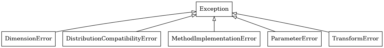
qmcpy.util.latnetbuilder_linker.latnetbuilder_linker(lnb_dir='./', out_dir='./', fout_prefix='lnb4qmcpy')

Parameters

lnb_dir (str) – relative path to directory where outputMachine.txt is stored e.g. ‘my_lnb/poly_lat/’
out_dir (str) – relative path to directory where output should be stored e.g. ‘my_lnb/poly_lat_qmcpy/’
fout_prefix (str) – start of output file name. e.g. ‘my_poly_lat_vec’

Returns

path to file which can be passed into QMCPy’s Lattice or Sobol’ in order to use: the linked latnetbuilder generating vector/matrix e.g. ‘my_poly_lat_vec.10.16.npy’

Return type

str

Adapted from latnetbuilder parser:: https://github.com/umontreal-simul/latnetbuilder/blob/master/python-wrapper/latnetbuilder/parse_output.py#L74