Monte Carlo for Vector Functions of Integrals
Demo Accompanying Aleksei Sorokin’s PyData Chicago 2023 Talk
Monte Carlo Problem
![\text{True Mean} = \mu = \mathbb{E}[g(T)] = \mathbb{E}[f(X)] = \int_{[0,1]^d} f(x) \mathrm{d} x \approx \frac{1}{n} \sum_{i=0}^{n-1} f(X_i) = \hat{\mu} = \text{Sample Mean}](../_images/math/c2f690349a6ab50e163d2d5d477a31ff1eef9ad1.png)
 , original measure on
 , original integrand
![X \sim \mathcal{U}[0,1]^d](../_images/math/c8fc0f1c81512b761b5d4d1e5bcc79d0ab904be6.png) , transformed measure
, transformed measure![f: [0,1]^d \to \mathbb{R}](../_images/math/bc32c989090e64b67363f0977f3098089e3c12c2.png) , transformed integrand
, transformed integrand
Python Setup
import qmcpy as qp
import numpy as np
import scipy.stats
import pandas as pd
import time
from matplotlib import pyplot
pyplot.style.use('../qmcpy/qmcpy.mplstyle')
colors = pyplot.rcParams['axes.prop_cycle'].by_key()['color']
%matplotlib inline
Discrete Distribution
Generate sampling locations
![X_0,\dots,X_{n-1} \sim \mathcal{U}[0,1]^d](../_images/math/bcaa0283ec270824dc1d74232ad7991a44a191e7.png)
Independent Identically Distributed (IID) Points for Crude Monte Carlo (CMC)
iid = qp.IIDStdUniform(dimension=3)
iid.gen_samples(n=4)
array([[0.33212887, 0.77514762, 0.32281907],
       [0.63606431, 0.87304412, 0.160779  ],
       [0.86648199, 0.16583253, 0.28605698],
       [0.33916281, 0.40836749, 0.59704801]])
iid.gen_samples(4)
array([[0.52964844, 0.93287387, 0.92878954],
       [0.52281122, 0.70201421, 0.23376703],
       [0.92408974, 0.69777308, 0.15770565],
       [0.33577149, 0.68206595, 0.97291222]])
iid
IIDStdUniform (DiscreteDistribution Object)
    d               3
    entropy         260382129008356013626800297715809294905
    spawn_key       ()
Low Discrepancy (LD) Points for Quasi-Monte Carlo (QMC)
ld_lattice = qp.Lattice(3)
ld_lattice.gen_samples(4)
array([[0.53421508, 0.29262606, 0.39547365],
       [0.03421508, 0.79262606, 0.89547365],
       [0.78421508, 0.04262606, 0.14547365],
       [0.28421508, 0.54262606, 0.64547365]])
ld_lattice.gen_samples(4)
array([[0.53421508, 0.29262606, 0.39547365],
       [0.03421508, 0.79262606, 0.89547365],
       [0.78421508, 0.04262606, 0.14547365],
       [0.28421508, 0.54262606, 0.64547365]])
ld_lattice.gen_samples(n_min=2,n_max=4)
array([[0.78421508, 0.04262606, 0.14547365],
       [0.28421508, 0.54262606, 0.64547365]])
ld_lattice
Lattice (DiscreteDistribution Object)
    d               3
    dvec            [0 1 2]
    randomize       1
    order           natural
    gen_vec         [     1 182667 469891]
    entropy         258997323036294594641435801210344083177
    spawn_key       ()
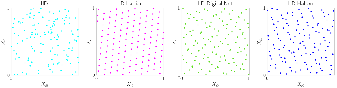
Visuals
IID vs LD Points
n = 2**7 # Lattice and Digital Net prefer powers of 2 sample sizes
discrete_distribs = {
    'IID': qp.IIDStdUniform(2),
    'LD Lattice': qp.Lattice(2),
    'LD Digital Net': qp.DigitalNetB2(2),
    'LD Halton': qp.Halton(2)}
fig,ax = pyplot.subplots(nrows=1,ncols=len(discrete_distribs),figsize=(3*len(discrete_distribs),3))
ax = np.atleast_1d(ax)
for i,(name,discrete_distrib) in enumerate(discrete_distribs.items()):
    x = discrete_distrib.gen_samples(n)
    ax[i].scatter(x[:,0],x[:,1],s=5,color=colors[i])
    ax[i].set_title(name)
    ax[i].set_aspect(1)
    ax[i].set_xlabel(r'$X_{i0}$'); ax[i].set_ylabel(r'$X_{i1}$')
    ax[i].set_xlim([0,1]); ax[i].set_ylim([0,1])
    ax[i].set_xticks([0,1]); ax[i].set_yticks([0,1])
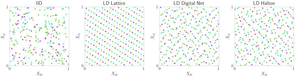
LD Space Filling Extensibility
m_min,m_max = 6,8
fig,ax = pyplot.subplots(nrows=1,ncols=len(discrete_distribs),figsize=(3*len(discrete_distribs),3))
ax = np.atleast_1d(ax)
for i,(name,discrete_distrib) in enumerate(discrete_distribs.items()):
    x = discrete_distrib.gen_samples(2**m_max)
    n_min = 0
    for m in range(m_min,m_max+1):
        n_max = 2**m
        ax[i].scatter(x[n_min:n_max,0],x[n_min:n_max,1],s=5,color=colors[m-m_min],label='n_min = %d, n_max = %d'%(n_min,n_max))
        n_min = 2**m
    ax[i].set_title(name)
    ax[i].set_aspect(1)
    ax[i].set_xlabel(r'$X_{i0}$'); ax[i].set_ylabel(r'$X_{i1}$')
    ax[i].set_xlim([0,1]); ax[i].set_ylim([0,1])
    ax[i].set_xticks([0,1]); ax[i].set_yticks([0,1])
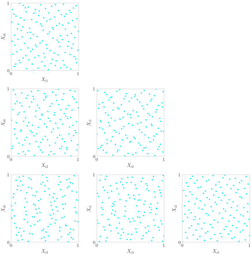
High Dimensional Pairs Plotting
discrete_distrib = qp.DigitalNetB2(4)
x = discrete_distrib(2**7)
d = discrete_distrib.d
assert d>=2
fig,ax = pyplot.subplots(nrows=d,ncols=d,figsize=(3*d,3*d))
for i in range(d):
    fig.delaxes(ax[i,i])
    for j in range(i):
        ax[i,j].scatter(x[:,i],x[:,j],s=5)
        fig.delaxes(ax[j,i])
        ax[i,j].set_aspect(1)
        ax[i,j].set_xlabel(r'$X_{i%d}$'%i); ax[i,j].set_ylabel(r'$X_{i%d}$'%j)
        ax[i,j].set_xlim([0,1]); ax[i,j].set_ylim([0,1])
        ax[i,j].set_xticks([0,1]); ax[i,j].set_yticks([0,1])
True Measure
Define , facilitate transform from original integrand  to transformed integrand
discrete_distrib = qp.Halton(3)
true_measure = qp.Gaussian(discrete_distrib,mean=[1,2,3],covariance=[4,5,6])
true_measure.gen_samples(4)
array([[ 0.40678465,  1.60773559,  0.34020435],
       [ 5.25849108,  3.60610932,  3.86999995],
       [ 1.42111148, -0.90377725,  2.30796197],
       [-0.8050952 ,  2.23293569,  5.98842354]])
true_measure.gen_samples(n_min=2,n_max=4)
array([[ 1.42111148, -0.90377725,  2.30796197],
       [-0.8050952 ,  2.23293569,  5.98842354]])
true_measure
Gaussian (TrueMeasure Object)
    mean            [1 2 3]
    covariance      [4 5 6]
    decomp_type     PCA
Visuals
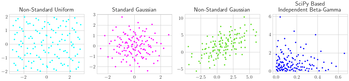
Some True Measure Samplings
n = 2**7
discrete_distrib = qp.DigitalNetB2(2)
true_measures = {
    'Non-Standard Uniform': qp.Uniform(discrete_distrib,lower_bound=[-3,-2],upper_bound=[3,2]),
    'Standard Gaussian': qp.Gaussian(discrete_distrib),
    'Non-Standard Gaussian': qp.Gaussian(discrete_distrib,mean=[1,2],covariance=[[5,4],[4,9]]),
    'SciPy Based\nIndependent Beta-Gamma': qp.SciPyWrapper(discrete_distrib,[scipy.stats.beta(a=1,b=5),scipy.stats.gamma(a=1)])}
fig,ax = pyplot.subplots(nrows=1,ncols=len(true_measures),figsize=(3*len(true_measures),3))
ax = np.atleast_1d(ax)
for i,(name,true_measure) in enumerate(true_measures.items()):
    t = true_measure.gen_samples(n)
    ax[i].scatter(t[:,0],t[:,1],s=5,color=colors[i])
    ax[i].set_title(name)
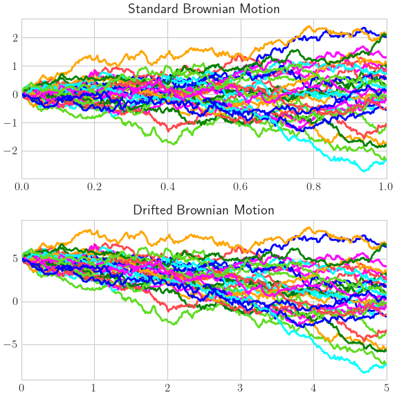
Brownian Motion
n = 32
discrete_distrib = qp.Lattice(365)
brownian_motions = {
    'Standard Brownian Motion': qp.BrownianMotion(discrete_distrib),
    'Drifted Brownian Motion': qp.BrownianMotion(discrete_distrib,t_final=5,initial_value=5,drift=-1,diffusion=2)}
fig,ax = pyplot.subplots(nrows=len(brownian_motions),ncols=1,figsize=(6,3*len(brownian_motions)))
ax = np.atleast_1d(ax)
for i,(name,brownian_motion) in enumerate(brownian_motions.items()):
    t = brownian_motion.gen_samples(n)
    t_w_init = np.hstack([brownian_motion.initial_value*np.ones((n,1)),t])
    tvec_w_0 = np.hstack([0,brownian_motion.time_vec])
    ax[i].plot(tvec_w_0,t_w_init.T)
    ax[i].set_xlim([tvec_w_0[0],tvec_w_0[-1]])
    ax[i].set_title(name)
Integrand
Define original integrand , store transformed integrand
Wrap your Function into QMCPy
Our simple example


![\mathbb{E}[f(X)] = \mathbb{E}[g(T)] = 0](../_images/math/f7b9d9ae791ba8538f7beded05b84efa646d3d8b.png)
def myfun(t): # define g, the ORIGINAL integrand
    # t an (n,d) shaped np.ndarray of sample from the ORIGINAL (true) measure
    y = t.sum(1)
    return y # an (n,) shaped np.ndarray
true_measure = qp.Gaussian(qp.Halton(5)) # LD Halton discrete distrib for QMC problem
qp_myfun = qp.CustomFun(true_measure,myfun,parallel=False)
Evalute the Automatically Transformed Integrand
x = qp_myfun.discrete_distrib.gen_samples(4) # samples from the TRANSFORMED measure
y = qp_myfun.f(x) # evaluate the TRANSFORMED integrand at the TRANSFORMED samples
y
array([[-3.28135198],
       [ 0.58308562],
       [-3.74555828],
       [ 3.35850654]])
Manual QMC Approximation
Note that when doing importance sampling the below doesn’t work. In that case we need to take a specially weighted sum instead instead of the equally weighted sum as done below.
x = qp_myfun.discrete_distrib.gen_samples(2**16) # samples from the TRANSFORMED measure
y = qp_myfun.f(x) # evaluate the TRANSFORMED integrand at the TRANSFORMED samples
mu_hat = y.mean()
mu_hat
-1.8119973887083317e-05
Predefined Integrands
Many more integrands detailed at https://qmcpy.readthedocs.io/en/master/algorithms.html#integrand-class
Integrands contain their true measure definition, so the user only needs to pass in a sampler. Samplers are often just discrete distributions.
asian_option = qp.AsianOption(
    sampler = qp.DigitalNetB2(52),
    volatility = 1/2,
    start_price = 30,
    strike_price = 35,
    interest_rate = 0.001,
    t_final = 1,
    call_put = 'call',
    mean_type = 'arithmetic')
x = asian_option.discrete_distrib.gen_samples(2**16)
y = asian_option.f(x)
mu_hat = y.mean()
mu_hat
1.7888072890178057
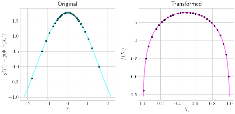
Visual Transformation
n = 32
keister = qp.Keister(qp.DigitalNetB2(1))
fig,ax = pyplot.subplots(nrows=1,ncols=2,figsize=(8,4))
x = keister.discrete_distrib.gen_samples(n)
t = keister.true_measure.gen_samples(n)
f_of_x = keister.f(x).squeeze()
g_of_t = keister.g(t).squeeze()
assert (f_of_x==g_of_t).all()
x_fine = np.linspace(0,1,257)[1:-1,None]
f_of_xfine = keister.f(x_fine).squeeze()
lb = 1.2*max(abs(t.min()),abs(t.max()))
t_fine = np.linspace(-lb,lb,257)[:,None]
g_of_tfine = keister.g(t_fine).squeeze()
ax[0].set_title(r'Original')
ax[0].set_xlabel(r'$T_i$'); ax[0].set_ylabel(r'$g(T_i) = g(\Phi^{-1}(X_i))$')
ax[0].plot(t_fine.squeeze(),g_of_tfine,color=colors[0],alpha=.5)
ax[0].scatter(t.squeeze(),f_of_x,s=10,color='k')
ax[1].set_title(r'Transformed')
ax[1].set_xlabel(r'$X_i$'); ax[1].set_ylabel(r'$f(X_i)$')
ax[1].scatter(x.squeeze(),f_of_x,s=10,color='k')
ax[1].plot(x_fine.squeeze(),f_of_xfine,color=colors[1],alpha=.5);
Stopping Criterion
Adaptively increase  until
until
 where
where
 is a user defined tolerance.
The stopping criterion should match the discrete distribution e.g. IID CMC stopping criterion for IID points, QMC Lattice stopping criterion for LD Lattice points, QMC digital net stopping criterion for LD digital net points, etc.
IID CMC Algorithm
problem_cmc = qp.AsianOption(qp.IIDStdUniform(52))
cmc_stop_crit = qp.CubMCG(problem_cmc,abs_tol=0.025)
approx_cmc,data_cmc = cmc_stop_crit.integrate()
data_cmc
MeanVarData (AccumulateData Object)
    solution        1.770
    error_bound     0.025
    n_total         445001
    n               443977
    levels          1
    time_integrate  2.678
CubMCG (StoppingCriterion Object)
    abs_tol         0.025
    rel_tol         0
    n_init          2^(10)
    n_max           10000000000
    inflate         1.200
    alpha           0.010
AsianOption (Integrand Object)
    volatility      2^(-1)
    call_put        call
    start_price     30
    strike_price    35
    interest_rate   0
    mean_type       arithmetic
    dim_frac        0
BrownianMotion (TrueMeasure Object)
    time_vec        [0.019 0.038 0.058 ... 0.962 0.981 1.   ]
    drift           0
    mean            [0. 0. 0. ... 0. 0. 0.]
    covariance      [[0.019 0.019 0.019 ... 0.019 0.019 0.019]
                    [0.019 0.038 0.038 ... 0.038 0.038 0.038]
                    [0.019 0.038 0.058 ... 0.058 0.058 0.058]
                    ...
                    [0.019 0.038 0.058 ... 0.962 0.962 0.962]
                    [0.019 0.038 0.058 ... 0.962 0.981 0.981]
                    [0.019 0.038 0.058 ... 0.962 0.981 1.   ]]
    decomp_type     PCA
IIDStdUniform (DiscreteDistribution Object)
    d               52
    entropy         61684358647256879138636107852151853477
    spawn_key       ()
LD QMC Algorithm
problem_qmc = qp.AsianOption(qp.DigitalNetB2(52))
qmc_stop_crit = qp.CubQMCNetG(problem_qmc,abs_tol=0.025)
approx_qmc,data_qmc = qmc_stop_crit.integrate()
data_qmc
LDTransformData (AccumulateData Object)
    solution        1.784
    comb_bound_low  1.759
    comb_bound_high 1.809
    comb_flags      1
    n_total         2^(10)
    n               2^(10)
    time_integrate  0.008
CubQMCNetG (StoppingCriterion Object)
    abs_tol         0.025
    rel_tol         0
    n_init          2^(10)
    n_max           2^(35)
AsianOption (Integrand Object)
    volatility      2^(-1)
    call_put        call
    start_price     30
    strike_price    35
    interest_rate   0
    mean_type       arithmetic
    dim_frac        0
BrownianMotion (TrueMeasure Object)
    time_vec        [0.019 0.038 0.058 ... 0.962 0.981 1.   ]
    drift           0
    mean            [0. 0. 0. ... 0. 0. 0.]
    covariance      [[0.019 0.019 0.019 ... 0.019 0.019 0.019]
                    [0.019 0.038 0.038 ... 0.038 0.038 0.038]
                    [0.019 0.038 0.058 ... 0.058 0.058 0.058]
                    ...
                    [0.019 0.038 0.058 ... 0.962 0.962 0.962]
                    [0.019 0.038 0.058 ... 0.962 0.981 0.981]
                    [0.019 0.038 0.058 ... 0.962 0.981 1.   ]]
    decomp_type     PCA
DigitalNetB2 (DiscreteDistribution Object)
    d               52
    dvec            [ 0  1  2 ... 49 50 51]
    randomize       LMS_DS
    graycode        0
    entropy         190424263390524682978874000220828251392
    spawn_key       ()
print('QMC took %.2f%% the time and %.2f%% the samples compared to CMC'%(
      100*data_qmc.time_integrate/data_cmc.time_integrate,100*data_qmc.n_total/data_cmc.n_total))
QMC took 0.29% the time and 0.23% the samples compared to CMC
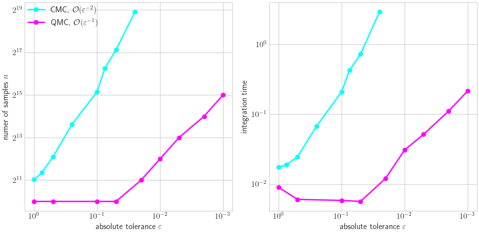
Visual CMC vs LD
cmc_tols = [1,.75,.5,.25,.1,.075,.05,.025]
qmc_tols = [1,.5,.1,.05,.02,.01,.005,.002,.001]
fig,ax = pyplot.subplots(nrows=1,ncols=2,figsize=(10,5))
n_cmc,time_cmc = np.zeros_like(cmc_tols),np.zeros_like(cmc_tols)
for i,cmc_tol in enumerate(cmc_tols):
    cmc_stop_crit = qp.CubMCG( qp.AsianOption(qp.IIDStdUniform(52)),abs_tol=cmc_tol)
    approx_cmc,data_cmc = cmc_stop_crit.integrate()
    n_cmc[i],time_cmc[i] = data_cmc.n_total,data_cmc.time_integrate
ax[0].plot(cmc_tols,n_cmc,'-o',color=colors[0],label=r'CMC, $\mathcal{O}(\varepsilon^{-2})$')
ax[1].plot(cmc_tols,time_cmc,'-o',color=colors[0])
n_qmc,time_qmc = np.zeros_like(qmc_tols),np.zeros_like(qmc_tols)
for i,qmc_tol in enumerate(qmc_tols):
    qmc_stop_crit = qp.CubQMCNetG(qp.AsianOption(qp.DigitalNetB2(52)),abs_tol=qmc_tol)
    approx_qmc,data_qmc = qmc_stop_crit.integrate()
    n_qmc[i],time_qmc[i] = data_qmc.n_total,data_qmc.time_integrate
ax[0].plot(qmc_tols,n_qmc,'-o',color=colors[1],label=r'QMC, $\mathcal{O}(\varepsilon^{-1})$')
ax[1].plot(qmc_tols,time_qmc,'-o',color=colors[1])
ax[0].set_xscale('log',base=10); ax[0].set_yscale('log',base=2)
ax[1].set_xscale('log',base=10); ax[1].set_yscale('log',base=10)
ax[0].invert_xaxis(); ax[1].invert_xaxis()
ax[0].set_xlabel(r'absolute tolerance $\varepsilon$'); ax[1].set_xlabel(r'absolute tolerance $\varepsilon$')
ax[0].set_ylabel(r'numer of samples $n$'); ax[1].set_ylabel('integration time')
ax[0].legend(loc='upper left');
Vectorized Stopping Criterion
Many more examples available at https://github.com/QMCSoftware/QMCSoftware/blob/master/demos/vectorized_qmc.ipynb
Vector of Expectations
As a simple example, lets compute
![\mathbb{E}[\cos(T_0)\cdots\cos(T_{d-1})]](../_images/math/0feec7dc3629360690a106da682c5b616d3a743a.png) and
and
![\mathbb{E}[\sin(T_0)\cdots\sin(T_{d-1})]](../_images/math/b2da8b81cef9b5e08b671d140e84029488de98d9.png) where
where
![T \sim \mathcal{U}[0,\pi]^d](../_images/math/35b631803c6a13b4aae454a3b0a98e34c5b49a46.png)
qmc_stop_crit = qp.CubQMCCLT(
    integrand = qp.CustomFun(
        true_measure = qp.Uniform(sampler=qp.Halton(3),lower_bound=0,upper_bound=np.pi),
        g = lambda t,compute_flags: np.vstack([np.cos(t).prod(1),np.sin(t).prod(1)]).T,
        dimension_indv = 2),
    abs_tol=.0001)
approx,data = qmc_stop_crit.integrate()
data
MeanVarDataRep (AccumulateData Object)
    solution        [2.534e-05 2.580e-01]
    comb_bound_low  [-6.766e-05  2.579e-01]
    comb_bound_high [1.183e-04 2.581e-01]
    comb_flags      [ True  True]
    n_total         2^(18)
    n               [262144.  65536.]
    n_rep           [16384.  4096.]
    time_integrate  0.194
CubQMCCLT (StoppingCriterion Object)
    inflate         1.200
    alpha           0.010
    abs_tol         1.00e-04
    rel_tol         0
    n_init          2^(8)
    n_max           2^(30)
    replications    2^(4)
CustomFun (Integrand Object)
Uniform (TrueMeasure Object)
    lower_bound     0
    upper_bound     3.142
Halton (DiscreteDistribution Object)
    d               3
    dvec            [0 1 2]
    randomize       QRNG
    generalize      1
    entropy         103520389532066966624097310655355259890
    spawn_key       ()
Covariance
In a simple example, let  and compute
the covariance of
and compute
the covariance of  and
and
 so that
![\mathrm{Cov}[P,S] = \mathbb{E}[PS]-\mathbb{E}[P]\mathbb{E}[S] = \mu_0-\mu_1\mu_2](../_images/math/40db8e33e65345c438953d04de653459425fd409.png)
Theoretically we have ![\mathrm{Cov}[P,S] = 2d-(1)(d) = d](../_images/math/92dceebe2a6d1b526917a974a49910b4e39f3fab.png)
class CovIntegrand(qp.integrand.Integrand):
    def __init__(self,sampler):
        self.sampler = sampler
        self.true_measure = qp.Gaussian(sampler,mean=1)
        super(CovIntegrand,self).__init__(dimension_indv=3,dimension_comb=1,parallel=False)
    def g(self, t, compute_flags):
        y = np.zeros((len(t),3))
        y[:,1] = t.prod(1) # P
        y[:,2] = t.sum(1) # S
        y[:,0] = y[:,1]*y[:,2] #PS
        return y
    def _spawn(self, level, sampler):
        return CovFun(sampler)
    def bound_fun(self, low, high):
        comb_low = low[0]-max(low[1]*low[2],low[1]*high[2],high[1]*low[2],high[1]*high[2])
        comb_high = high[0]-min(low[1]*low[2],low[1]*high[2],high[1]*low[2],high[1]*high[2])
        return comb_low,comb_high
    def dependency(self, comb_flag):
        return np.tile(comb_flag,3)
approx,data = qp.CubQMCLatticeG(CovIntegrand(qp.Lattice(10)),rel_tol=.025).integrate()
data
LDTransformData (AccumulateData Object)
    solution        9.889
    comb_bound_low  9.697
    comb_bound_high 10.090
    comb_flags      1
    n_total         2^(20)
    n               [1048576. 1048576. 1048576.]
    time_integrate  3.316
CubQMCLatticeG (StoppingCriterion Object)
    abs_tol         0.010
    rel_tol         0.025
    n_init          2^(10)
    n_max           2^(35)
CovIntegrand (Integrand Object)
Gaussian (TrueMeasure Object)
    mean            1
    covariance      1
    decomp_type     PCA
Lattice (DiscreteDistribution Object)
    d               10
    dvec            [0 1 2 3 4 5 6 7 8 9]
    randomize       1
    order           natural
    gen_vec         [     1 182667 469891 498753 110745 446247 250185 118627 245333 283199]
    entropy         333426925650737605782635567565068085620
    spawn_key       ()
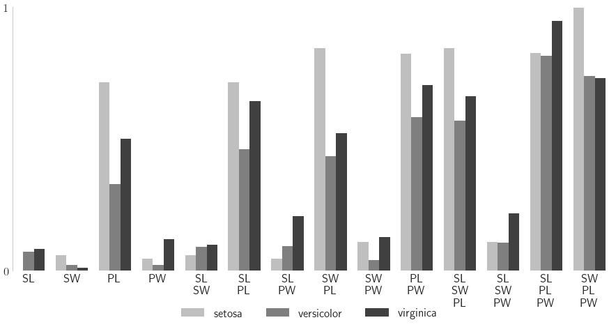
Sensitiviy Indices
See Appendix A of Art Owen’s Monte Carlo Book
In the following example, we fit a neural network to Iris flower features and try to classify the Iris species. For each set of features, the classifier provides a probability of belonging to each species, a length 3 vector. We quantify the sensitiviy of this classificaiton probability to Iris features, assuming features are uniformly distributed throughout the feature domain.
from sklearn.datasets import load_iris
from sklearn.model_selection import train_test_split
from sklearn.neural_network import MLPClassifier
data = load_iris()
og_feature_names = data["feature_names"]
feature_names = [fn.replace('sepal ','S')\
    .replace('length ','L')\
    .replace('petal ','P')\
    .replace('width ','W')\
    .replace('(cm)','') for fn in og_feature_names]
target_names = data["target_names"]
xt,xv,yt,yv = train_test_split(data["data"],data["target"],
    test_size = 1/3,
    random_state = 7)
pd.DataFrame(np.hstack([data['data'],data['target'][:,None]]),columns=og_feature_names+['species']).iloc[[0,1,90,91,140,141]]
| sepal length (cm) | sepal width (cm) | petal length (cm) | petal width (cm) | species | |
|---|---|---|---|---|---|
| 0 | 5.1 | 3.5 | 1.4 | 0.2 | 0.0 |
| 1 | 4.9 | 3.0 | 1.4 | 0.2 | 0.0 |
| 90 | 5.5 | 2.6 | 4.4 | 1.2 | 1.0 |
| 91 | 6.1 | 3.0 | 4.6 | 1.4 | 1.0 |
| 140 | 6.7 | 3.1 | 5.6 | 2.4 | 2.0 |
| 141 | 6.9 | 3.1 | 5.1 | 2.3 | 2.0 |
mlpc = MLPClassifier(random_state=7,max_iter=1024).fit(xt,yt)
yhat = mlpc.predict(xv)
print("accuracy: %.1f%%"%(100*(yv==yhat).mean()))
# accuracy: 98.0%
sampler = qp.DigitalNetB2(4,seed=7)
true_measure =  qp.Uniform(sampler,
    lower_bound = xt.min(0),
    upper_bound = xt.max(0))
fun = qp.CustomFun(
    true_measure = true_measure,
    g = lambda x,compute_flags: mlpc.predict_proba(x),
    dimension_indv = 3)
si_fun = qp.SensitivityIndices(fun,indices="all")
qmc_algo = qp.CubQMCNetG(si_fun,abs_tol=.005)
nn_sis,nn_sis_data = qmc_algo.integrate()
accuracy: 98.0%
#print(nn_sis_data.flags_indv.shape)
#print(nn_sis_data.flags_comb.shape)
print('samples: 2^(%d)'%np.log2(nn_sis_data.n_total))
print('time: %.1e'%nn_sis_data.time_integrate)
print('indices:',nn_sis_data.integrand.indices)

import pandas as pd

df_closed = pd.DataFrame(nn_sis[0],columns=target_names,index=[str(idx) for idx in nn_sis_data.integrand.indices])
print('\nClosed Indices')
print(df_closed)
df_total = pd.DataFrame(nn_sis[1],columns=target_names,index=[str(idx) for idx in nn_sis_data.integrand.indices])
print('\nTotal Indices')
print(df_total)
df_closed_singletons = df_closed.T.iloc[:,:4]
df_closed_singletons['sum singletons'] = df_closed_singletons[['[%d]'%i for i in range(4)]].sum(1)
df_closed_singletons.columns = data['feature_names']+['sum']
df_closed_singletons = df_closed_singletons*100
samples: 2^(15)
time: 1.6e+00
indices: [[0], [1], [2], [3], [0, 1], [0, 2], [0, 3], [1, 2], [1, 3], [2, 3], [0, 1, 2], [0, 1, 3], [0, 2, 3], [1, 2, 3]]

Closed Indices
             setosa  versicolor  virginica
[0]        0.001504    0.071122   0.081736
[1]        0.058743    0.022073   0.010373
[2]        0.713777    0.328313   0.500059
[3]        0.046053    0.021077   0.120233
[0, 1]     0.059178    0.091764   0.098233
[0, 2]     0.715117    0.460138   0.642551
[0, 3]     0.046859    0.092322   0.207724
[1, 2]     0.843241    0.434629   0.520469
[1, 3]     0.108872    0.039572   0.127844
[2, 3]     0.823394    0.582389   0.705354
[0, 1, 2]  0.845359    0.570022   0.661100
[0, 1, 3]  0.108503    0.106081   0.218971
[0, 2, 3]  0.825389    0.814286   0.948331
[1, 2, 3]  0.996483    0.738213   0.729940

Total Indices
             setosa  versicolor  virginica
[0]        0.003199    0.259762   0.265085
[1]        0.172391    0.183159   0.045582
[2]        0.889677    0.896874   0.780377
[3]        0.157794    0.433342   0.340092
[0, 1]     0.174905    0.414246   0.289565
[0, 2]     0.890477    0.966238   0.871992
[0, 3]     0.159744    0.566187   0.478082
[1, 2]     0.949190    0.907994   0.790445
[1, 3]     0.283542    0.540486   0.355714
[2, 3]     0.941651    0.919005   0.902203
[0, 1, 2]  0.949431    0.980367   0.880283
[0, 1, 3]  0.284118    0.674406   0.497364
[0, 2, 3]  0.942185    0.986186   0.989555
[1, 2, 3]  0.996057    0.933342   0.913711
nindices = len(nn_sis_data.integrand.indices)
fig,ax = pyplot.subplots(figsize=(9,5))
ticks = np.arange(nindices)
width = .25
for i,(alpha,species) in enumerate(zip([.25,.5,.75],data['target_names'])):
    cvals = df_closed[species].to_numpy()
    tvals = df_total[species].to_numpy()
    ticks_i = ticks+i*width
    ax.bar(ticks_i,cvals,width=width,align='edge',color='k',alpha=alpha,label=species)
    #ax.bar(ticks_i,np.flip(tvals),width=width,align='edge',bottom=1-np.flip(tvals),color=color,alpha=.1)
ax.set_xlim([0,13+3*width])
ax.set_xticks(ticks+1.5*width)

# closed_labels = [r'$\underline{s}_{\{%s\}}$'%(','.join([r'\text{%s}'%feature_names[i] for i in idx])) for idx in nn_sis_data.integrand.indices]
closed_labels = ['\n'.join([feature_names[i] for i in idx]) for idx in nn_sis_data.integrand.indices]
ax.set_xticklabels(closed_labels,rotation=0)
ax.set_ylim([0,1]); ax.set_yticks([0,1])
ax.grid(False)
for spine in ['top','right','bottom']: ax.spines[spine].set_visible(False)
ax.legend(frameon=False,loc='lower center',bbox_to_anchor=(.5,-.2),ncol=3);