ML Sensitivity Indices
This notebook demonstrates QMCPy’s support for vectorized sensitivity index computation. We preview this functionality by performing classification of Iris species using a decision tree. The computed sensitivity indices provide insight into input subset importance for a classic machine learning problem.
from numpy import *
from qmcpy import *
import pandas as pd
from sklearn.datasets import load_iris
from sklearn.tree import DecisionTreeClassifier,plot_tree
from sklearn.model_selection import train_test_split
from skopt import gp_minimize
from matplotlib import pyplot
Load Data
We begin by reading in the Iris dataset and providing some basic summary statistics. Our goal will be to predict the Iris class (Setosa, Versicolour, or Virginica) based on Iris attributes (sepal length, sepal width, petal length, and petal width).
data = load_iris()
print(data['DESCR'])
.. _iris_dataset:

Iris plants dataset
--------------------

Data Set Characteristics:

    :Number of Instances: 150 (50 in each of three classes)
    :Number of Attributes: 4 numeric, predictive attributes and the class
    :Attribute Information:
        - sepal length in cm
        - sepal width in cm
        - petal length in cm
        - petal width in cm
        - class:
                - Iris-Setosa
                - Iris-Versicolour
                - Iris-Virginica

    :Summary Statistics:

    ============== ==== ==== ======= ===== ====================
                    Min  Max   Mean    SD   Class Correlation
    ============== ==== ==== ======= ===== ====================
    sepal length:   4.3  7.9   5.84   0.83    0.7826
    sepal width:    2.0  4.4   3.05   0.43   -0.4194
    petal length:   1.0  6.9   3.76   1.76    0.9490  (high!)
    petal width:    0.1  2.5   1.20   0.76    0.9565  (high!)
    ============== ==== ==== ======= ===== ====================

    :Missing Attribute Values: None
    :Class Distribution: 33.3% for each of 3 classes.
    :Creator: R.A. Fisher
    :Donor: Michael Marshall (MARSHALL%PLU@io.arc.nasa.gov)
    :Date: July, 1988

The famous Iris database, first used by Sir R.A. Fisher. The dataset is taken
from Fisher's paper. Note that it's the same as in R, but not as in the UCI
Machine Learning Repository, which has two wrong data points.

This is perhaps the best known database to be found in the
pattern recognition literature.  Fisher's paper is a classic in the field and
is referenced frequently to this day.  (See Duda & Hart, for example.)  The
data set contains 3 classes of 50 instances each, where each class refers to a
type of iris plant.  One class is linearly separable from the other 2; the
latter are NOT linearly separable from each other.

.. topic:: References

   - Fisher, R.A. "The use of multiple measurements in taxonomic problems"
     Annual Eugenics, 7, Part II, 179-188 (1936); also in "Contributions to
     Mathematical Statistics" (John Wiley, NY, 1950).
   - Duda, R.O., & Hart, P.E. (1973) Pattern Classification and Scene Analysis.
     (Q327.D83) John Wiley & Sons.  ISBN 0-471-22361-1.  See page 218.
   - Dasarathy, B.V. (1980) "Nosing Around the Neighborhood: A New System
     Structure and Classification Rule for Recognition in Partially Exposed
     Environments".  IEEE Transactions on Pattern Analysis and Machine
     Intelligence, Vol. PAMI-2, No. 1, 67-71.
   - Gates, G.W. (1972) "The Reduced Nearest Neighbor Rule".  IEEE Transactions
     on Information Theory, May 1972, 431-433.
   - See also: 1988 MLC Proceedings, 54-64.  Cheeseman et al"s AUTOCLASS II
     conceptual clustering system finds 3 classes in the data.
   - Many, many more ...
x = data['data']
y = data['target']
feature_names = data['feature_names']
df = pd.DataFrame(hstack((x,y[:,None])),columns=feature_names+['iris type'])
print('df shape:',df.shape)
target_names = data['target_names']
iris_type_map = {i:target_names[i] for i in range(len(target_names))}
print('iris species map:',iris_type_map)
df.head()
df shape: (150, 5)
iris species map: {0: 'setosa', 1: 'versicolor', 2: 'virginica'}
| sepal length (cm) | sepal width (cm) | petal length (cm) | petal width (cm) | iris type | |
|---|---|---|---|---|---|
| 0 | 5.1 | 3.5 | 1.4 | 0.2 | 0.0 |
| 1 | 4.9 | 3.0 | 1.4 | 0.2 | 0.0 |
| 2 | 4.7 | 3.2 | 1.3 | 0.2 | 0.0 |
| 3 | 4.6 | 3.1 | 1.5 | 0.2 | 0.0 |
| 4 | 5.0 | 3.6 | 1.4 | 0.2 | 0.0 |
xt,xv,yt,yv = train_test_split(x,y,test_size=1/3,random_state=7)
print('training data   (xt) shape: %s'%str(xt.shape))
print('training labels (yt) shape: %s'%str(yt.shape))
print('testing data    (xv) shape: %s'%str(xv.shape))
print('testing labels  (yv) shape: %s'%str(yv.shape))
training data   (xt) shape: (100, 4)
training labels (yt) shape: (100,)
testing data    (xv) shape: (50, 4)
testing labels  (yv) shape: (50,)
Importance of Decision Tree Hyperparameters
We would like to predict Iris species using a Decision Tree (DT) classifier. When initializing a DT, we arrive at the question of how to set hyperparameters such as tree depth or the minimum weight fraction for each leaf. These hyperparameters can greatly effect classification accuracy, so it is worthwhile to consider their importance to determining classification performance.
Note that while this notebook uses decision trees and the Iris dataset, the methodology is directly applicable to other datasets and models.
We begin this exploration by setting up a hyperparameter domain in which to uniformly sample DT hyperparameter configurations. A helper function and its tie into QMCPy are also created.
hp_domain = [
    {'name':'max_depth', 'bounds':[1,8]},
    {'name':'min_weight_fraction_leaf', 'bounds':[0,.5]}]
hpnames = [param['name'] for param in hp_domain]
hp_lb = array([param['bounds'][0] for param in hp_domain])
hp_ub = array([param['bounds'][1] for param in hp_domain])
d = len(hp_domain)
def get_dt_accuracy(hparams):
    accuracies = zeros(len(hparams))
    for i,hparam in enumerate(hparams):
        kwargs = {hp_domain[j]['name']:hparam[j] for j in range(d)}
        kwargs['max_depth'] = int(kwargs['max_depth'])
        dt = DecisionTreeClassifier(random_state=7,**kwargs).fit(xt,yt)
        yhat = dt.predict(xv)
        accuracies[i] = mean(yhat==yv)
    return accuracies
cf = CustomFun(
    true_measure = Uniform(DigitalNetB2(d,seed=7),lower_bound=hp_lb,upper_bound=hp_ub),
    g = get_dt_accuracy,
    parallel=False)
Average Accuracy
Our first goal will be to find the average DT accuracy across the hyperparameter domain. To do so, we perform quasi-Monte Carlo numerical integration to approximate the mean testing accuracy.
avg_accuracy,data_avg_accuracy = CubQMCNetG(cf,abs_tol=1e-4).integrate()
data_avg_accuracy
LDTransformData (AccumulateData Object)
    solution        0.787
    comb_bound_low  0.787
    comb_bound_high 0.787
    comb_flags      1
    n_total         2^(14)
    n               2^(14)
    time_integrate  8.745
CubQMCNetG (StoppingCriterion Object)
    abs_tol         1.00e-04
    rel_tol         0
    n_init          2^(10)
    n_max           2^(35)
CustomFun (Integrand Object)
Uniform (TrueMeasure Object)
    lower_bound     [1 0]
    upper_bound     [8.  0.5]
DigitalNetB2 (DiscreteDistribution Object)
    d               2^(1)
    dvec            [0 1]
    randomize       LMS_DS
    graycode        0
    entropy         7
    spawn_key       ()
Here we find the average accuracy to be 78.7% using  samples.
Sensitivity Indices
Next, we wish to quantify how important individual hyperparamters are to
determining testing accuracy. To do this, we compute the sensitivity
indices of our hyperparameters. In QMCPy we use the
SensitivityIndices class to compute these sensitivity indices.
si = SensitivityIndices(cf)
solution_importances,data_importances = CubQMCNetG(si,abs_tol=2.5e-2).integrate()
data_importances
LDTransformData (AccumulateData Object)
    solution        [[0.164 0.747]
                    [0.257 0.837]]
    comb_bound_low  [[0.148 0.726]
                    [0.238 0.819]]
    comb_bound_high [[0.179 0.768]
                    [0.277 0.856]]
    comb_flags      [[ True  True]
                    [ True  True]]
    n_total         2^(13)
    n               [[[4096. 8192.]
                     [4096. 8192.]
                     [4096. 8192.]]

                    [[2048. 8192.]
                     [2048. 8192.]
                     [2048. 8192.]]]
    time_integrate  14.999
CubQMCNetG (StoppingCriterion Object)
    abs_tol         0.025
    rel_tol         0
    n_init          2^(10)
    n_max           2^(35)
SensitivityIndices (Integrand Object)
    indices         [[0]
                    [1]]
    n_multiplier    2^(1)
Uniform (TrueMeasure Object)
    lower_bound     [1 0]
    upper_bound     [8.  0.5]
DigitalNetB2 (DiscreteDistribution Object)
    d               4
    dvec            [0 1 2 3]
    randomize       LMS_DS
    graycode        0
    entropy         7
    spawn_key       (0,)
print('closed sensitivity indices: %s'%str(solution_importances[0].squeeze()))
print('total sensitivity indices: %s'%str(solution_importances[1].squeeze()))
closed sensitivity indices: [0.16375873 0.74701157]
total sensitivity indices: [0.25724624 0.83732705]
Looking closer at the output, we see that the second hyperparameter
(min_weight_fraction_leaf) is more important than the first one
(max_depth). The closed sensitivity indices measure how much that
hyperparameter contributes to testing accuracy variance. The total
sensitivity indices measure how much that hyperparameter, or any subset
of hyperparameters containing that one contributes to testing accuracy
variance. For example, the first closed sensitivity index approximates
the variability attributable to {max_depth} while the first total
sensitivity index approximates the variability attributable to both
{max_depth} and {max_depth,min_weight_fraction_leaf}.
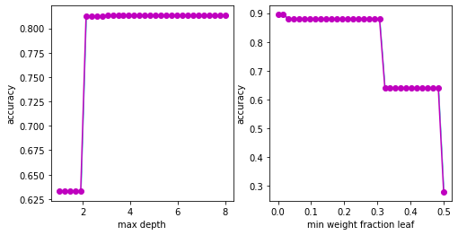
Marginals
We may also use QMCPy’s support for vectorized quasi-Monte Carlo to compute marginal distributions. This is relatively straightforward to do for the Uniform true measure used here, but caution should be taken when adapting these techniques to distributions without independent marginals.
def marginal(x,compute_flags,xpts,bools,not_bools):
    n,_ = x.shape
    x2 = zeros((n,d),dtype=float)
    x2[:,bools] = x
    y = zeros((n,len(xpts)),dtype=float)
    for k,xpt in enumerate(xpts):
        if not compute_flags[k]: continue
        x2[:,not_bools] = xpt
        y[:,k] = get_dt_accuracy(x2)
    return y
fig,ax = pyplot.subplots(nrows=1,ncols=2,figsize=(8,4))
nticks = 32
xpts01 = linspace(0,1,nticks)
for i in range(2):
    xpts = xpts01*(hp_ub[i]-hp_lb[i])+hp_lb[i]
    bools = array([True if j not in [i] else False for j in range(d)])
    def marginal_i(x,compute_flags): return marginal(x,compute_flags,xpts,bools,~bools)
    cf = CustomFun(
         true_measure = Uniform(DigitalNetB2(1,seed=7),lower_bound=hp_lb[bools],upper_bound=hp_ub[bools]),
         g = marginal_i,
         dimension_indv = len(xpts),
         parallel=False)
    sol,data = CubQMCNetG(cf,abs_tol=5e-2).integrate()
    ax[i].plot(xpts,sol,'-o',color='m')
    ax[i].fill_between(xpts,data.comb_bound_high,data.comb_bound_low,color='c',alpha=.5)
    ax[i].set_xlabel(hpnames[i].replace('_',' '))
    ax[i].set_ylabel('accuracy')
Bayesian Optimization of Hyperparameters
Having explored DT hyperparameter importance, we are now ready to construct our optimal DT. We already have quite a bit of data relating hyperparameter settings to testing accuracy, so we may simply select the best configuration and call this an optimal DT. However, if we are looking to squeeze out even more performance, we may choose to perform Bayesian Optimization which incorporates our past metadata. Sample code is provided below despite not finding an improved configuration for this problem.
x0 = data_avg_accuracy.xfull*(hp_ub-hp_lb)+hp_lb
y0 = -data_avg_accuracy.yfull.squeeze()
print('best result before BO is %d%% accuracy'%(-100*y0.min()))
result = gp_minimize(
    func = lambda hparams: get_dt_accuracy(atleast_2d(hparams)).squeeze().item(),
    dimensions = [(l,u) for l,u in zip(hp_lb,hp_ub)],
    n_calls = 32,
    n_initial_points = 0,
    x0 = x0[:128].tolist(),
    y0 = y0[:128].tolist(),
    random_state = 7)
xbo_best = result.x
ybo_best = -result.fun
print('best result from BO is %d%% accuracy'%(100*ybo_best))
xbo = array(result.x_iters)
ybo = -array(result.func_vals)
best result before BO is 94% accuracy
best result from BO is 94% accuracy
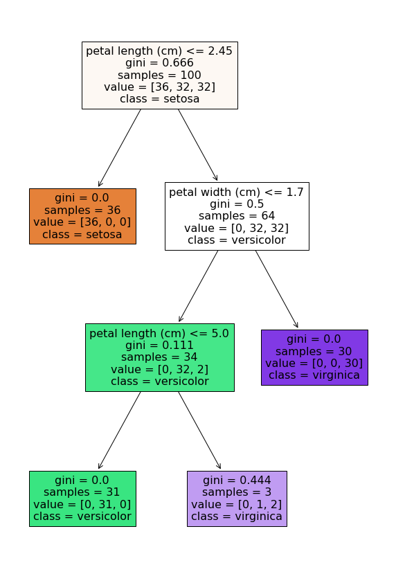
Best Decision Tree Analysis
Below we print the configuration that rested in the best DT. We also print the optimal accuracy achieved (at this configuration) and visualize the branches of this tree.
best_kwargs = {name:val for name,val in zip(hpnames,xbo_best)}
best_kwargs['max_depth'] = int(best_kwargs['max_depth'])
print(best_kwargs)
dt = DecisionTreeClassifier(random_state=7,**best_kwargs).fit(xt,yt)
yhat = dt.predict(xv)
accuracy = mean(yhat==yv)
print('best decision tree accuracy: %.1f%%'%(100*accuracy))
fig = pyplot.figure(figsize=(10,15))
plot_tree(dt,feature_names=feature_names,class_names=target_names,filled=True);
{'max_depth': 6, 'min_weight_fraction_leaf': 0.01750528148841113}
best decision tree accuracy: 94.0%
Feature Importance
With the optimal DT in hand, we may now question how important the Irises features are in determining the class/species. To answer this question, we again perform sensitivity analysis, but this time we select a uniform measure over the domain of Iris features. Our output which we wish to quantify the variance of is now a length 3 vector of class probabilities. How variable is each species classification as a function of each Iris feature?
xfeatures = df.to_numpy()
xfeatures_low = xfeatures[:,:-1].min(0)
xfeatures_high = xfeatures[:,:-1].max(0)
d_features = len(xfeatures_low)
def dt_pp(t,compute_flags): return dt.predict_proba(t)
cf = CustomFun(
    true_measure = Uniform(DigitalNetB2(d_features,seed=7),
        lower_bound = xfeatures_low,
        upper_bound = xfeatures_high),
    g = dt_pp,
    dimension_indv = 3,
    parallel = False)
indices = [[0],[1],[2],[3],[0,1],[0,2],[0,3],[1,2],[1,3],[2,3],[1,2,3],[0,2,3],[0,1,2]]
si_cf = SobolIndices(cf,indices)
solution,data = CubQMCNetG(si_cf,abs_tol=1e-3,n_init=2**10).integrate()
data
LDTransformData (AccumulateData Object)
    solution        [[[0.    0.    0.   ]
                     [0.    0.    0.   ]
                     [0.999 0.43  0.456]
                     ...
                     [0.999 0.999 1.   ]
                     [0.999 0.999 1.   ]
                     [0.999 0.43  0.456]]

                    [[0.    0.    0.   ]
                     [0.    0.    0.   ]
                     [1.    0.646 0.662]
                     ...
                     [1.    0.999 0.999]
                     [1.    0.999 0.999]
                     [1.    0.646 0.662]]]
    comb_bound_low  [[[0.    0.    0.   ]
                     [0.    0.    0.   ]
                     [0.999 0.43  0.455]
                     ...
                     [0.999 0.998 0.999]
                     [0.999 0.998 0.999]
                     [0.999 0.43  0.455]]

                    [[0.    0.    0.   ]
                     [0.    0.    0.   ]
                     [0.999 0.645 0.661]
                     ...
                     [0.999 0.998 0.999]
                     [0.999 0.998 0.999]
                     [0.999 0.645 0.661]]]
    comb_bound_high [[[0.    0.    0.   ]
                     [0.    0.    0.   ]
                     [1.    0.431 0.457]
                     ...
                     [1.    1.    1.   ]
                     [1.    1.    1.   ]
                     [1.    0.431 0.457]]

                    [[0.    0.    0.   ]
                     [0.    0.    0.   ]
                     [1.    0.647 0.662]
                     ...
                     [1.    1.    1.   ]
                     [1.    1.    1.   ]
                     [1.    0.647 0.662]]]
    comb_flags      [[[ True  True  True]
                     [ True  True  True]
                     [ True  True  True]
                     ...
                     [ True  True  True]
                     [ True  True  True]
                     [ True  True  True]]

                    [[ True  True  True]
                     [ True  True  True]
                     [ True  True  True]
                     ...
                     [ True  True  True]
                     [ True  True  True]
                     [ True  True  True]]]
    n_total         2^(17)
    n               [[[[  1024.   1024.   1024.]
                      [  1024.   1024.   1024.]
                      [  8192. 131072.  65536.]
                      ...
                      [  8192.  65536.  32768.]
                      [  8192.  65536.  32768.]
                      [  8192. 131072.  65536.]]

                     [[  1024.   1024.   1024.]
                      [  1024.   1024.   1024.]
                      [  8192. 131072.  65536.]
                      ...
                      [  8192.  65536.  32768.]
                      [  8192.  65536.  32768.]
                      [  8192. 131072.  65536.]]]


                    [[[  1024.   1024.   1024.]
                      [  1024.   1024.   1024.]
                      [  8192.  65536.  65536.]
                      ...
                      [  8192.  32768.  16384.]
                      [  8192.  32768.  16384.]
                      [  8192.  65536.  65536.]]

                     [[  1024.   1024.   1024.]
                      [  1024.   1024.   1024.]
                      [  8192.  65536.  65536.]
                      ...
                      [  8192.  32768.  16384.]
                      [  8192.  32768.  16384.]
                      [  8192.  65536.  65536.]]]]
    time_integrate  3.418
CubQMCNetG (StoppingCriterion Object)
    abs_tol         0.001
    rel_tol         0
    n_init          2^(10)
    n_max           2^(35)
SobolIndices (Integrand Object)
    indices         [[0], [1], [2], [3], [0, 1], [0, 2], [0, 3], [1, 2], [1, 3], [2, 3], [1, 2, 3], [0, 2, 3], [0, 1, 2]]
    n_multiplier    13
Uniform (TrueMeasure Object)
    lower_bound     [4.3 2.  1.  0.1]
    upper_bound     [7.9 4.4 6.9 2.5]
DigitalNetB2 (DiscreteDistribution Object)
    d               8
    dvec            [0 1 2 3 4 5 6 7]
    randomize       LMS_DS
    graycode        0
    entropy         7
    spawn_key       (0,)
While the solution looks unwieldy, it has quite a natural
interpretation. The first axis determines whether we are looking at a
closed (index 0) or total (index 1) sensitivity index as before. The
second axis indexes the subset of features we are testing. The third and
final axis is length 3 for the 3 class probabilities we are interested
in. For example, solution[0,2,2] looks at the closed sensitivity
index of our index 2 feature (petal length) for our index 2 probability
(virginica) AKA how important is petal length alone to determining if an
Iris is virginica.
The results indicate that setosa Irises can be completely determined based on petal length while the versicolor and virginica Irises can be completely determined by looking at both petal length and petal width. Interestingly sepal length and sepal width do not contribute significantly to determining species.
These insights are not surprising or especially insightful for a decision tree where the tree structure indicates importance and the scores may even be computed directly. However, for more complicated models and datasets, this analysis pipeline may provide advanced insight into both hyperparameter tuning and feature importance.
print('solution shape:',solution.shape,'\n')
si_closed = solution[0]
si_total = solution[1]
print('SI Closed')
print(si_closed,'\n')
print('SI Total')
print(si_total)
solution shape: (2, 13, 3)

SI Closed
[[0.         0.         0.        ]
 [0.         0.         0.        ]
 [0.99938581 0.43048672 0.45606325]
 [0.         0.35460247 0.33840028]
 [0.         0.         0.        ]
 [0.99938581 0.43048672 0.45606325]
 [0.         0.35460247 0.33840028]
 [0.99938581 0.43048672 0.45606325]
 [0.         0.35460247 0.33840028]
 [0.99938581 0.99922725 0.99970515]
 [0.99938581 0.99922725 0.99970515]
 [0.99938581 0.99922725 0.99970515]
 [0.99938581 0.43048672 0.45606325]]

SI Total
[[0.         0.         0.        ]
 [0.         0.         0.        ]
 [0.9996645  0.64566888 0.66160745]
 [0.         0.56908397 0.54359418]
 [0.         0.         0.        ]
 [0.9996645  0.64566888 0.66160745]
 [0.         0.56908397 0.54359418]
 [0.9996645  0.64566888 0.66160745]
 [0.         0.56908397 0.54359418]
 [0.9996645  0.99903766 0.99927206]
 [0.9996645  0.99903766 0.99927206]
 [0.9996645  0.99903766 0.99927206]
 [0.9996645  0.64566888 0.66160745]]
