Importance Sampling Examples

from qmcpy import *
from numpy import *
import pandas as pd
pd.options.display.float_format = '{:.2e}'.format
from matplotlib import pyplot as plt
import matplotlib
%matplotlib inline

Game Example

Consider a game where $X_1, X_2 \overset{\textrm{IID}}{\sim} \mathcal{U}(0,1)$ are drawn with a payoff of

$Y = \text{payoff}(X_1,X_2) = \begin{cases} \$10, & 1.7 \le X_1 + X_2 \le 2, \\ 0, & 0 \le X_1 + X_2 < 1.7, \end{cases}$

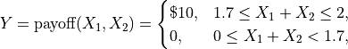
What is the expected payoff of this game?

payoff = lambda x: 10*(x.sum(1)>1.7)
abs_tol = 1e-3

Vanilla Monte Carlo

With ordinary Monte Carlo we do the following:

$\mu = \mathbb{E}(Y) = \int_{[0,1]^2} \text{payoff}(x_1,x_2) \, \mathrm{d} x_1 \mathrm{d}x_2$

d = 2
integral = CustomFun(
    true_measure = Uniform(Lattice(d)),
    g = payoff)
solution1,data1 = CubQMCLatticeG(integral, abs_tol).integrate()
data1

LDTransformData (AccumulateData Object)
    solution        0.450
    comb_bound_low  0.449
    comb_bound_high 0.450
    comb_flags      1
    n_total         2^(16)
    n               2^(16)
    time_integrate  0.043
CubQMCLatticeG (StoppingCriterion Object)
    abs_tol         0.001
    rel_tol         0
    n_init          2^(10)
    n_max           2^(35)
CustomFun (Integrand Object)
Uniform (TrueMeasure Object)
    lower_bound     0
    upper_bound     1
Lattice (DiscreteDistribution Object)
    d               2^(1)
    dvec            [0 1]
    randomize       1
    order           natural
    entropy         260768472417330885254602359583380448047
    spawn_key       ()

Monte Carlo with Importance Sampling

We may add the importance sampling to increase the number of samples with positive payoffs. Let

$\boldsymbol{Z} = (X_1^{1/(p+1)}, X_2^{1/(p+1)}), \qquad \boldsymbol{X} \sim \mathcal{U}(0,1)^2$

This means that $Z_1$ and $Z_2$ are IID with common CDF $F(z) =z^{p+1}$ and common PDF $\varrho(z) = (p+1)z^{p}$ . Thus,

$\mu = \mathbb{E}(Y) = \int_{[0,1]^2} \frac{\text{payoff}(z_1,z_2)}{(p+1)^2(z_1z_2)^{p}} \, \varrho(z_1) \varrho(z_2) \, \mathrm{d} z_1 \mathrm{d}z_2 \\ = \int_{[0,1]^2} \frac{\text{payoff}(x_1^{1/(p+1)},x_2^{1/(p+1)})}{(p+1)^2(x_1x_2)^{p/(p+1)}} \, \mathrm{d} x_1 \mathrm{d}x_2$

p = 1
d = 2
integral = CustomFun(
    true_measure = Uniform(Lattice(d)),
    g = lambda x: payoff(x**(1/(p+1))) / ((p+1)**2 * (x.prod(1))**(p/(p+1))))
solution2,data2 = CubQMCLatticeG(integral, abs_tol).integrate()
data2

LDTransformData (AccumulateData Object)
    solution        0.451
    comb_bound_low  0.450
    comb_bound_high 0.451
    comb_flags      1
    n_total         2^(14)
    n               2^(14)
    time_integrate  0.019
CubQMCLatticeG (StoppingCriterion Object)
    abs_tol         0.001
    rel_tol         0
    n_init          2^(10)
    n_max           2^(35)
CustomFun (Integrand Object)
Uniform (TrueMeasure Object)
    lower_bound     0
    upper_bound     1
Lattice (DiscreteDistribution Object)
    d               2^(1)
    dvec            [0 1]
    randomize       1
    order           natural
    entropy         101794984569737015308869089738144162915
    spawn_key       ()

print('Imporance Sampling takes %.3f the time and %.3f the samples'%\
     (data2.time_integrate/data1.time_integrate,data2.n_total/data1.n_total))

Imporance Sampling takes 0.451 the time and 0.250 the samples

Asian Call Option Example

The stock price must raise significantly for the payoff to be positive. So we will give an upward drift to the Brownian motion that defines the stock price path. We can think of the option price as the multidimensional integral

$\mu = \mathbb{E}[f(\boldsymbol{X})] = \int_{\mathbb{R}^d} f(\boldsymbol{x}) \frac{\exp\bigl(-\frac{1}{2} \boldsymbol{x}^T\mathsf{\Sigma}^{-1} \boldsymbol{x}\bigr)} {\sqrt{(2 \pi)^{d} \det(\mathsf{\Sigma})}} \, \mathrm{d} \boldsymbol{x}$

where

$\boldsymbol{X} \sim \mathcal{N}(\boldsymbol{0}, \mathsf{\Sigma}), \qquad \mathsf{\Sigma} = \bigl(\min(j,k)T/d \bigr)_{j,k=1}^d, \qquad d = 13, \\ f(\boldsymbol{x}) = \max\biggl(K - \frac 1d \sum_{j=1}^d S(jT/d,\boldsymbol{x}), 0 \biggr) \mathrm{e}^{-rT}, \\ S(jT/d,\boldsymbol{x}) = S(0) \exp\bigl((r - \sigma^2/2) jT/d + \sigma x_j\bigr).$

We will replace $\boldsymbol{X}$ by

$\boldsymbol{Z} \sim \mathcal{N}(\boldsymbol{a}, \mathsf{\Sigma}), \qquad \boldsymbol{a} = (aT/d)(1, \ldots, d)$

where a positive $a$ will create more positive payoffs. This corresponds to giving our Brownian motion a drift. To do this we re-write the integral as

$\mu = \mathbb{E}[f_{\mathrm{new}}(\boldsymbol{Z})] = \int_{\mathbb{R}^d} f_{\mathrm{new}}(\boldsymbol{z}) \frac{\exp\bigl(-\frac{1}{2} (\boldsymbol{z}-\boldsymbol{a})^T \mathsf{\Sigma}^{-1} (\boldsymbol{z} - \boldsymbol{a}) \bigr)} {\sqrt{(2 \pi)^{d} \det(\mathsf{\Sigma})}} \, \mathrm{d} \boldsymbol{z} , \\ f_{\mathrm{new}}(\boldsymbol{z}) = f(\boldsymbol{z}) \frac{\exp\bigl(-\frac{1}{2} \boldsymbol{z}^T \mathsf{\Sigma}^{-1} \boldsymbol{z} \bigr)} {\exp\bigl(-\frac{1}{2} (\boldsymbol{z}-\boldsymbol{a})^T \mathsf{\Sigma}^{-1} (\boldsymbol{z} - \boldsymbol{a}) \bigr)} = f(\boldsymbol{z}) \exp\bigl((\boldsymbol{a}/2 - \boldsymbol{z})^T \mathsf{\Sigma}^{-1}\boldsymbol{a} \bigr)$

Finally note that

$\mathsf{\Sigma}^{-1}\boldsymbol{a} = \begin{pmatrix} 0 \\ 0 \\ \vdots \\ 0 \\ a \end{pmatrix}, \qquad f_{\mathrm{new}}(\boldsymbol{z}) = f(\boldsymbol{z}) \exp\bigl((aT/2 - z_d)a \bigr)$

This drift in the Brownian motion may be implemented by changing the drift input to the BrownianMotion object.

abs_tol = 1e-2
dimension = 32

Vanilla Monte Carlo

integrand = AsianOption(Sobol(dimension))
solution1,data1 = CubQMCSobolG(integrand, abs_tol).integrate()
data1

LDTransformData (AccumulateData Object)
    solution        1.788
    comb_bound_low  1.782
    comb_bound_high 1.794
    comb_flags      1
    n_total         2^(12)
    n               2^(12)
    time_integrate  0.014
CubQMCSobolG (StoppingCriterion Object)
    abs_tol         0.010
    rel_tol         0
    n_init          2^(10)
    n_max           2^(35)
AsianOption (Integrand Object)
    volatility      2^(-1)
    call_put        call
    start_price     30
    strike_price    35
    interest_rate   0
    mean_type       arithmetic
    dim_frac        0
BrownianMotion (TrueMeasure Object)
    time_vec        [0.031 0.062 0.094 ... 0.938 0.969 1.   ]
    drift           0
    mean            [0. 0. 0. ... 0. 0. 0.]
    covariance      [[0.031 0.031 0.031 ... 0.031 0.031 0.031]
                    [0.031 0.062 0.062 ... 0.062 0.062 0.062]
                    [0.031 0.062 0.094 ... 0.094 0.094 0.094]
                    ...
                    [0.031 0.062 0.094 ... 0.938 0.938 0.938]
                    [0.031 0.062 0.094 ... 0.938 0.969 0.969]
                    [0.031 0.062 0.094 ... 0.938 0.969 1.   ]]
    decomp_type     PCA
Sobol (DiscreteDistribution Object)
    d               2^(5)
    dvec            [ 0  1  2 ... 29 30 31]
    randomize       LMS_DS
    graycode        0
    entropy         296048682239793520955192894339316320391
    spawn_key       ()

Monte Carlo with Importance Sampling

drift = 1
integrand = AsianOption(BrownianMotion(Sobol(dimension),drift=drift))
solution2,data2 = CubQMCSobolG(integrand, abs_tol).integrate()
data2

LDTransformData (AccumulateData Object)
    solution        1.783
    comb_bound_low  1.776
    comb_bound_high 1.790
    comb_flags      1
    n_total         2^(11)
    n               2^(11)
    time_integrate  0.014
CubQMCSobolG (StoppingCriterion Object)
    abs_tol         0.010
    rel_tol         0
    n_init          2^(10)
    n_max           2^(35)
AsianOption (Integrand Object)
    volatility      2^(-1)
    call_put        call
    start_price     30
    strike_price    35
    interest_rate   0
    mean_type       arithmetic
    dim_frac        0
BrownianMotion (TrueMeasure Object)
    time_vec        [0.031 0.062 0.094 ... 0.938 0.969 1.   ]
    drift           0
    mean            [0. 0. 0. ... 0. 0. 0.]
    covariance      [[0.031 0.031 0.031 ... 0.031 0.031 0.031]
                    [0.031 0.062 0.062 ... 0.062 0.062 0.062]
                    [0.031 0.062 0.094 ... 0.094 0.094 0.094]
                    ...
                    [0.031 0.062 0.094 ... 0.938 0.938 0.938]
                    [0.031 0.062 0.094 ... 0.938 0.969 0.969]
                    [0.031 0.062 0.094 ... 0.938 0.969 1.   ]]
    decomp_type     PCA
    transform       BrownianMotion (TrueMeasure Object)
                       time_vec        [0.031 0.062 0.094 ... 0.938 0.969 1.   ]
                       drift           1
                       mean            [0.031 0.062 0.094 ... 0.938 0.969 1.   ]
                       covariance      [[0.031 0.031 0.031 ... 0.031 0.031 0.031]
                                       [0.031 0.062 0.062 ... 0.062 0.062 0.062]
                                       [0.031 0.062 0.094 ... 0.094 0.094 0.094]
                                       ...
                                       [0.031 0.062 0.094 ... 0.938 0.938 0.938]
                                       [0.031 0.062 0.094 ... 0.938 0.969 0.969]
                                       [0.031 0.062 0.094 ... 0.938 0.969 1.   ]]
                       decomp_type     PCA
Sobol (DiscreteDistribution Object)
    d               2^(5)
    dvec            [ 0  1  2 ... 29 30 31]
    randomize       LMS_DS
    graycode        0
    entropy         144971093458566807495711477416245436939
    spawn_key       ()

print('Imporance Sampling takes %.3f the time and %.3f the samples'%\
     (data2.time_integrate/data1.time_integrate,data2.n_total/data1.n_total))

Imporance Sampling takes 1.009 the time and 0.500 the samples

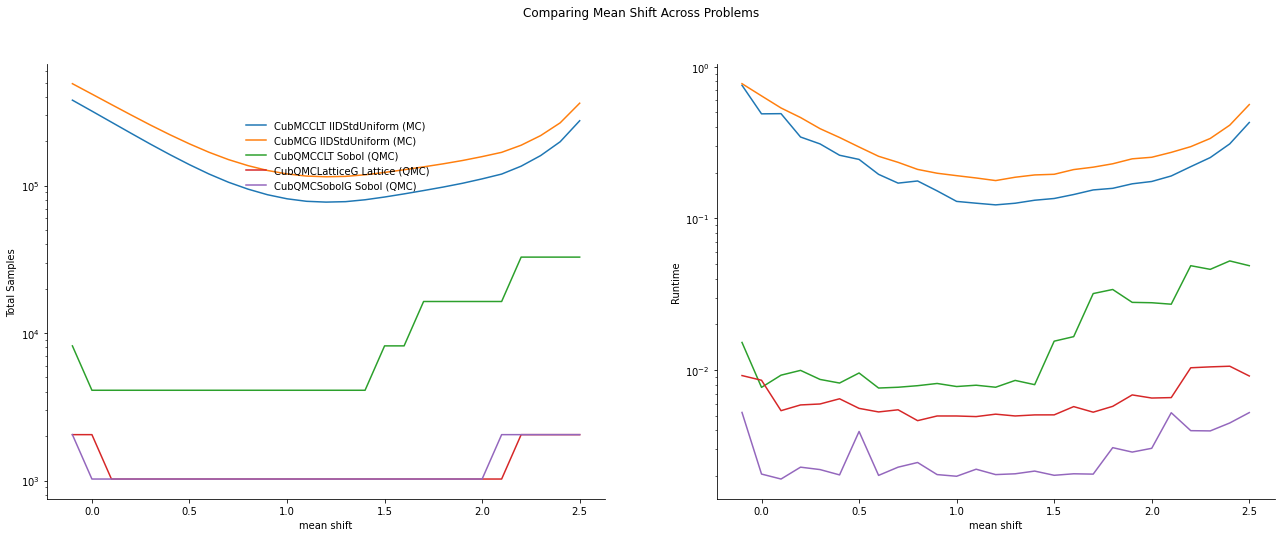
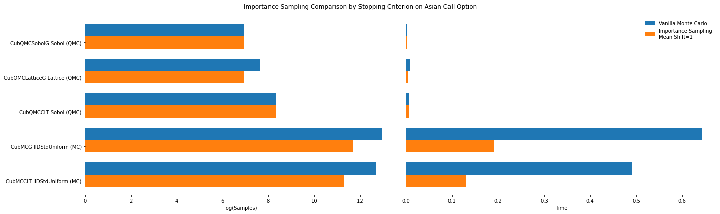
Importance Sampling MC vs QMC

Test Parameters

dimension = 16
abs_tol = .025
trials = 3

df = pd.read_csv('../workouts/mc_vs_qmc/out/importance_sampling.csv')
df['Problem'] = df['Stopping Criterion'] + ' ' + df['Distribution'] + ' (' + df['MC/QMC'] + ')'
df = df.drop(['Stopping Criterion','Distribution','MC/QMC'],axis=1)
problems = ['CubMCCLT IIDStdUniform (MC)',
            'CubMCG IIDStdUniform (MC)',
            'CubQMCCLT Sobol (QMC)',
            'CubQMCLatticeG Lattice (QMC)',
            'CubQMCSobolG Sobol (QMC)']
df = df[df['Problem'].isin(problems)]
mean_shifts = df.mean_shift.unique()
df_samples = df.groupby(['Problem'])['n_samples'].apply(list).reset_index(name='n')
df_times = df.groupby(['Problem'])['time'].apply(list).reset_index(name='time')
df.loc[(df.mean_shift==0) | (df.mean_shift==1)].set_index('Problem')
# Note: mean_shift==0 --> NOT using importance sampling

	mean_shift	solution	n_samples	time
Problem
CubMCCLT IIDStdUniform (MC)	0.00e+00	1.80e+00	3.20e+05	4.90e-01
CubMCCLT IIDStdUniform (MC)	1.00e+00	1.77e+00	8.15e+04	1.30e-01
CubMCG IIDStdUniform (MC)	0.00e+00	1.80e+00	4.18e+05	6.43e-01
CubMCG IIDStdUniform (MC)	1.00e+00	1.77e+00	1.20e+05	1.91e-01
CubQMCCLT Sobol (QMC)	0.00e+00	1.78e+00	4.10e+03	7.69e-03
CubQMCCLT Sobol (QMC)	1.00e+00	1.78e+00	4.10e+03	7.79e-03
CubQMCLatticeG Lattice (QMC)	0.00e+00	1.78e+00	2.05e+03	8.56e-03
CubQMCLatticeG Lattice (QMC)	1.00e+00	1.78e+00	1.02e+03	4.98e-03
CubQMCSobolG Sobol (QMC)	0.00e+00	1.78e+00	1.02e+03	2.06e-03
CubQMCSobolG Sobol (QMC)	1.00e+00	1.78e+00	1.02e+03	1.99e-03

fig,ax = plt.subplots(nrows=1, ncols=2, figsize=(20, 6))
idx = arange(len(problems))
width = .35
ax[0].barh(idx+width,log(df.loc[df.mean_shift==0]['n_samples'].values),width)
ax[0].barh(idx,log(df.loc[df.mean_shift==1]['n_samples'].values),width)
ax[1].barh(idx+width,df.loc[df.mean_shift==0]['time'].values,width)
ax[1].barh(idx,df.loc[df.mean_shift==1]['time'].values,width)
fig.suptitle('Importance Sampling Comparison by Stopping Criterion on Asian Call Option')
xlabs = ['log(Samples)','Time']
for i in range(len(ax)):
    ax[i].set_xlabel(xlabs[i])
    ax[i].spines['top'].set_visible(False)
    ax[i].spines['bottom'].set_visible(False)
    ax[i].spines['right'].set_visible(False)
    ax[i].spines['left'].set_visible(False)
    ax[1].legend(['Vanilla Monte Carlo','Importance Sampling\nMean Shift=1'],loc='upper right',frameon=False)
ax[1].get_yaxis().set_ticks([])
ax[0].set_yticks(idx)
ax[0].set_yticklabels(problems)
plt.tight_layout();

fig,ax = plt.subplots(nrows=1, ncols=2, figsize=(22, 8))
df_samples.apply(lambda row: ax[0].plot(mean_shifts,row.n,label=row['Problem']),axis=1)
df_times.apply(lambda row: ax[1].plot(mean_shifts,row.time,label=row['Problem']),axis=1)
ax[1].legend(frameon=False, loc=(-.85,.7),ncol=1)
ax[0].set_ylabel('Total Samples')
ax[0].set_yscale('log')
ax[1].set_yscale('log')
ax[1].set_ylabel('Runtime')
for i in range(len(ax)):
    ax[i].set_xlabel('mean shift')
    ax[i].spines['top'].set_visible(False)
    ax[i].spines['right'].set_visible(False)
fig.suptitle('Comparing Mean Shift Across Problems');