Gaussian Diagnostics

Experiments to demonstate Guassian assumption used in cubBayesLattice

import numpy as np
import matplotlib.pyplot as plt
from scipy.optimize import fmin as fminsearch
from numpy import prod, sin, cos, pi
from scipy.stats import norm as gaussnorm
from matplotlib import cm

from qmcpy.integrand import Keister
from qmcpy.discrete_distribution.lattice import Lattice

# print(plt.style.available)
# plt.style.use('./presentation.mplstyle')  # use custom settings
plt.style.use('seaborn-poster')

# plt.rcParams.update({'font.size': 12})
# plt.rcParams.update({'lines.linewidth': 2})
# plt.rcParams.update({'lines.markersize': 6})

Let us define the objective function. (cubBayesLattice) finds optimal parameters by minimizing the objective function

def ObjectiveFunction(theta, order, xun, ftilde):
    tol = 100 * np.finfo(float).eps
    n = len(ftilde)
    arbMean = True
    Lambda = kernel2(theta, order, xun)

    # compute RKHSnorm
    # temp = abs(ftilde(Lambda  != 0).^ 2)./ (Lambda(Lambda != 0))
    temp = abs(ftilde[Lambda > tol] ** 2) / (Lambda[Lambda > tol])

    # compute loss: MLE
    if arbMean == True:
        RKHSnorm = sum(temp[1:]) / n
        temp_1 = sum(temp[1:])
    else:
        RKHSnorm = sum(temp) / n
        temp_1 = sum(temp)

    # ignore all zero eigenvalues
    loss1 = sum(np.log(Lambda[Lambda > tol])) / n
    loss2 = np.log(temp_1)
    loss = (loss1 + loss2)
    if np.imag(loss) != 0:
        # keyboard
        raise('error ! : loss value is complex')

    # print('L1 %1.3f L2 %1.3f L %1.3f r %1.3e theta %1.3e\n'.format(loss1, loss2, loss, order, theta))
    return loss, Lambda, RKHSnorm

Series approximation of the shift invariant kernel

def kernel2(theta, r, xun):
    n = xun.shape[0]
    m = np.arange(1, (n / 2))
    tilde_g_h1 = m ** (-r)
    tilde_g = np.hstack([0, tilde_g_h1, 0, tilde_g_h1[::-1]])
    g = np.fft.fft(tilde_g)
    temp_ = (theta / 2) * g[(xun * n).astype(int)]
    C1 = prod(1 + temp_, 1)
    # eigenvalues must be real : Symmetric pos definite Kernel
    vlambda = np.real(np.fft.fft(C1))
    return vlambda

Gaussian random function

def f_rand(xpts, rfun, a, b, c, seed):
    dim = xpts.shape[1]
    np.random.seed(seed)  # initialize random number generator for reproducability
    N1 = int(2 ** np.floor(16 / dim))
    Nall = N1 ** dim
    kvec = np.zeros([dim, Nall])  # initialize kvec
    kvec[0, 0:N1] = range(0, N1)  # first dimension
    Nd = N1
    for d in range(1, dim):
        Ndm1 = Nd
        Nd = Nd * N1
        kvec[0:d+1, 0:Nd] = np.vstack([
            np.tile(kvec[0:d, 0:Ndm1], (1, N1)),
            np.reshape(np.tile(np.arange(0, N1), (Ndm1, 1)), (1, Nd), order="F")
        ])

    kvec = kvec[:, 1: Nall]  # remove the zero wavenumber
    whZero = np.sum(kvec == 0, axis=0)
    abfac = a ** (dim - whZero) * b ** whZero
    kbar = np.prod(np.maximum(kvec, 1), axis=0)
    totfac = abfac / (kbar ** rfun)

    f_c = a * np.random.randn(1, Nall - 1) * totfac
    f_s = a * np.random.randn(1, Nall - 1) * totfac

    f_0 = c + (b ** dim) * np.random.randn()
    argx = np.matmul((2 * np.pi * xpts), kvec)
    f_c_ = f_c * np.cos(argx)
    f_s_ = f_s * np.sin(argx)
    fval = f_0 + np.sum(f_c_ + f_s_, axis=1)
    return fval

Periodization transforms

def doPeriodTx(x, integrand, ptransform):
    ptransform = ptransform.upper()
    if ptransform == 'BAKER':  # Baker's transform
        xp = 1 - 2 * abs(x - 1 / 2)
        w = 1
    elif ptransform == 'C0':  # C^0 transform
        xp = 3 * x ** 2 - 2 * x ** 3
        w = prod(6 * x * (1 - x), 1)
    elif ptransform == 'C1':  # C^1 transform
        xp = x ** 3 * (10 - 15 * x + 6 * x ** 2)
        w = prod(30 * x ** 2 * (1 - x) ** 2, 1)
    elif ptransform == 'C1SIN':  # Sidi C^1 transform
        xp = x - sin(2 * pi * x) / (2 * pi)
        w = prod(2 * sin(pi * x) ** 2, 1)
    elif ptransform == 'C2SIN':  # Sidi C^2 transform
        xp = (8 - 9 * cos(pi * x) + cos(3 * pi * x)) / 16  # psi3
        w = prod((9 * sin(pi * x) * pi - sin(3 * pi * x) * 3 * pi) / 16, 1)  # psi3_1
    elif ptransform == 'C3SIN':  # Sidi C^3 transform
        xp = (12 * pi * x - 8 * sin(2 * pi * x) + sin(4 * pi * x)) / (12 * pi)  # psi4
        w = prod((12 * pi - 8 * cos(2 * pi * x) * 2 * pi + sin(4 * pi * x) * 4 * pi) / (12 * pi), 1)  # psi4_1
    elif ptransform == 'NONE':
        xp = x
        w = 1
    else:
        raise (f"The {ptransform} periodization transform is not implemented")
    y = integrand(xp) * w
    return y

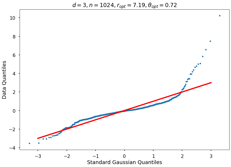
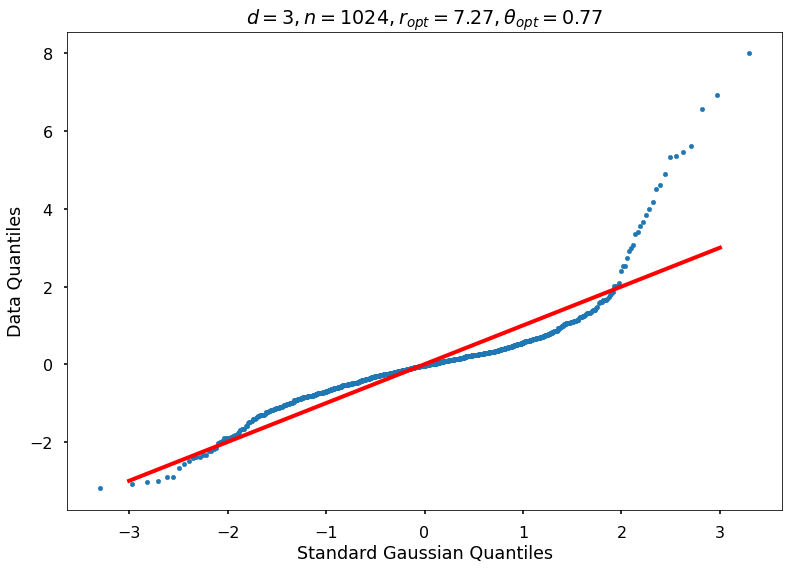
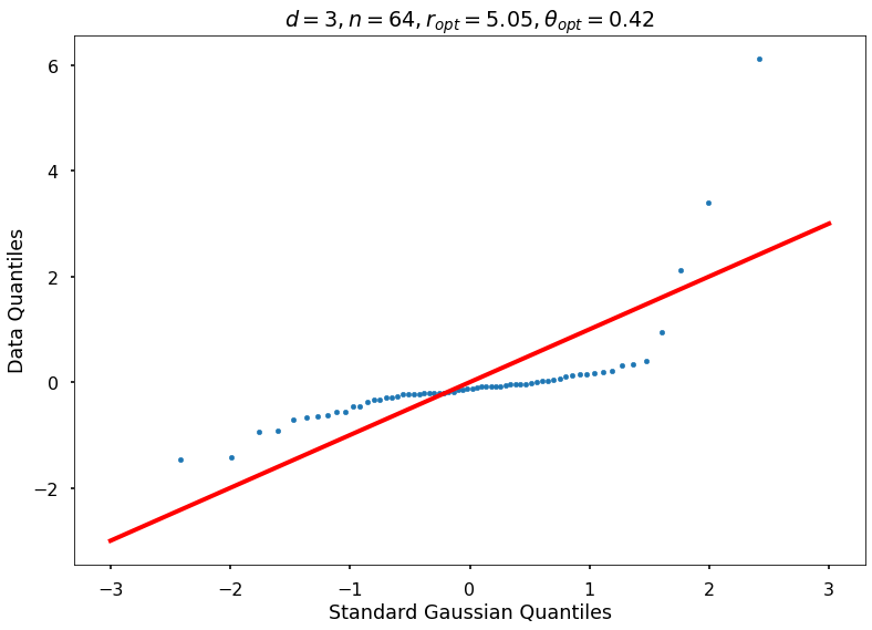
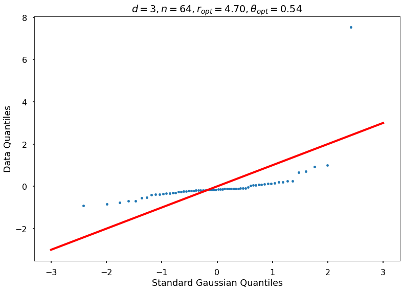
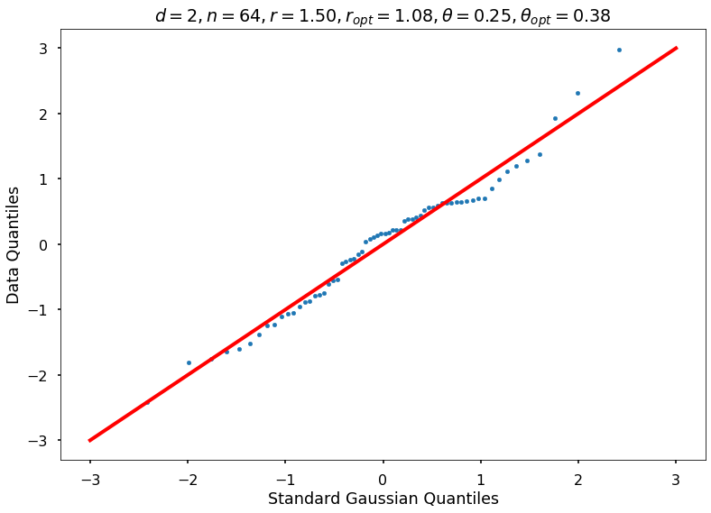
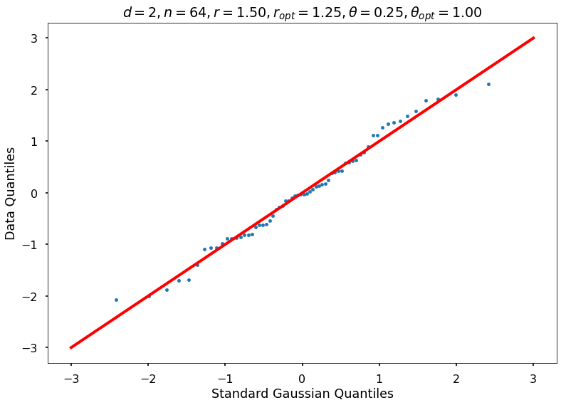
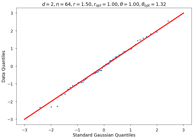
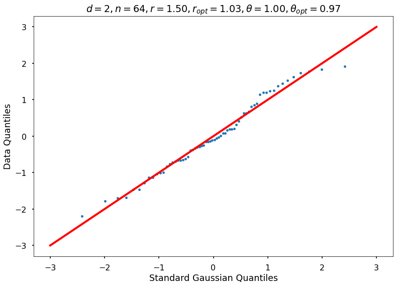
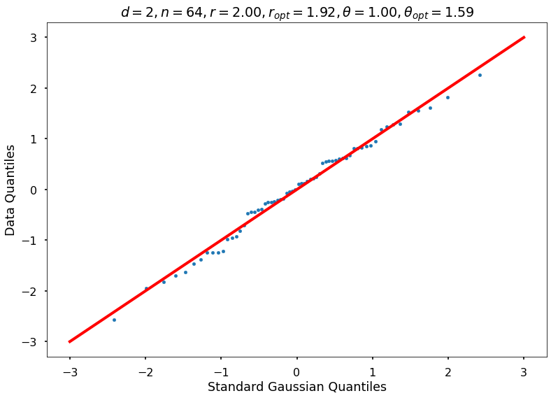
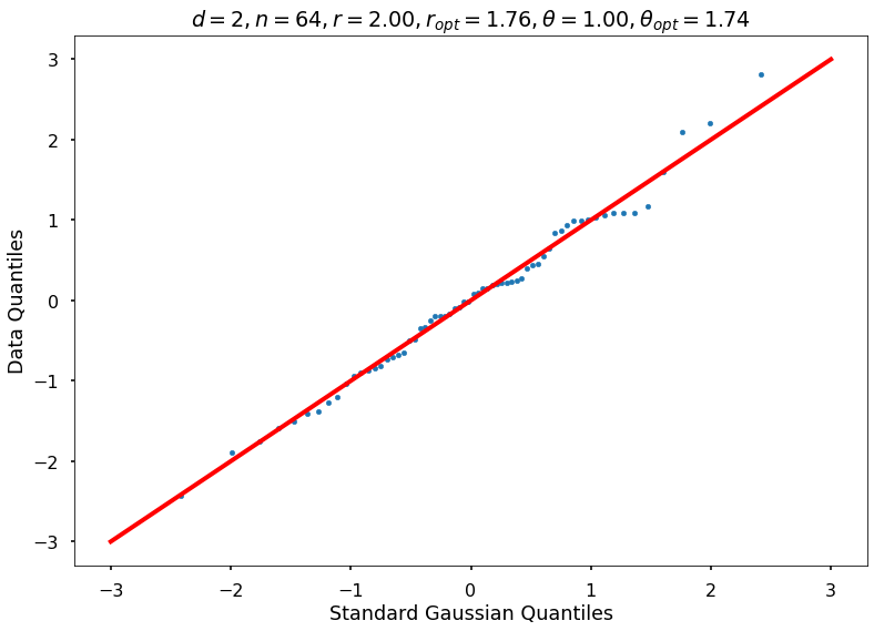
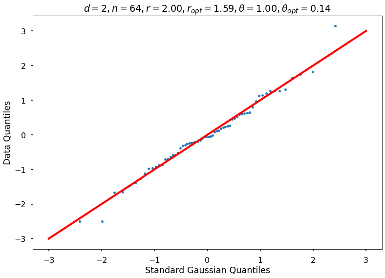
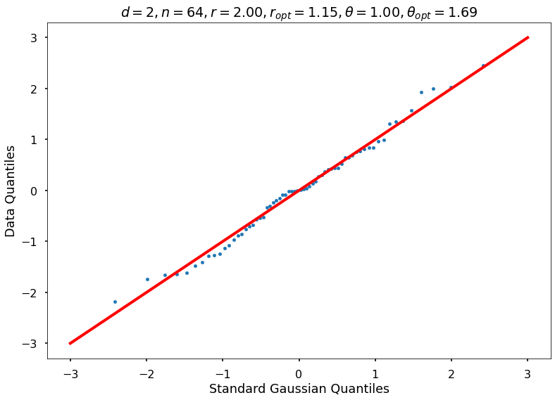
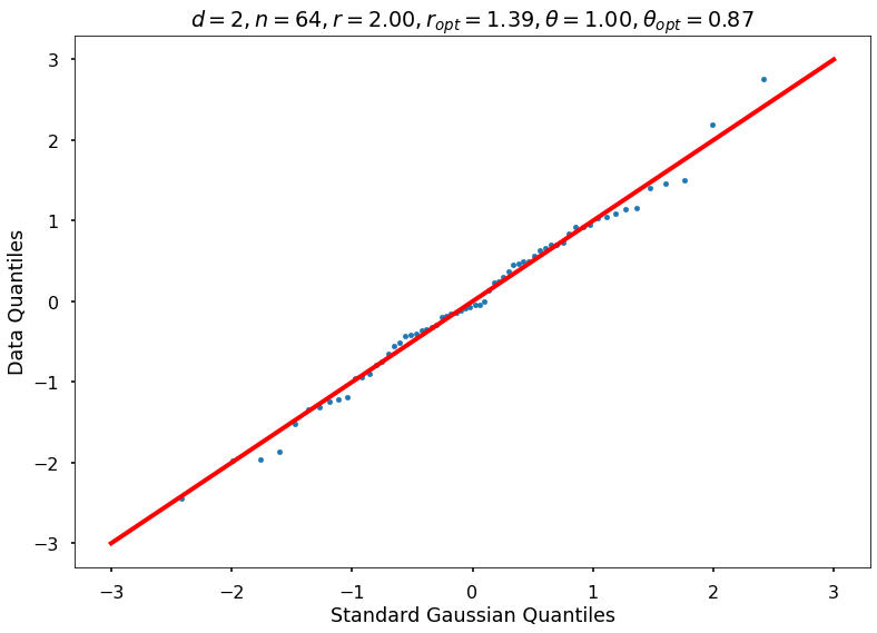
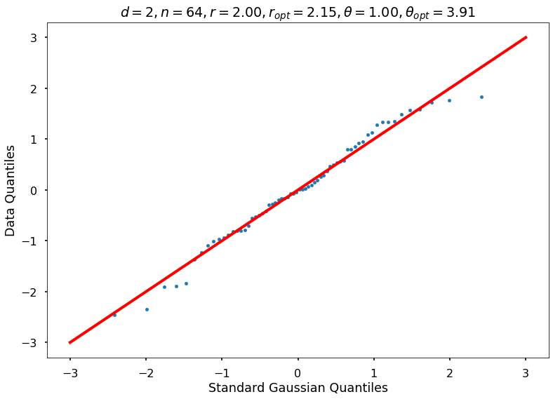
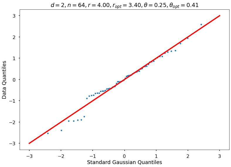
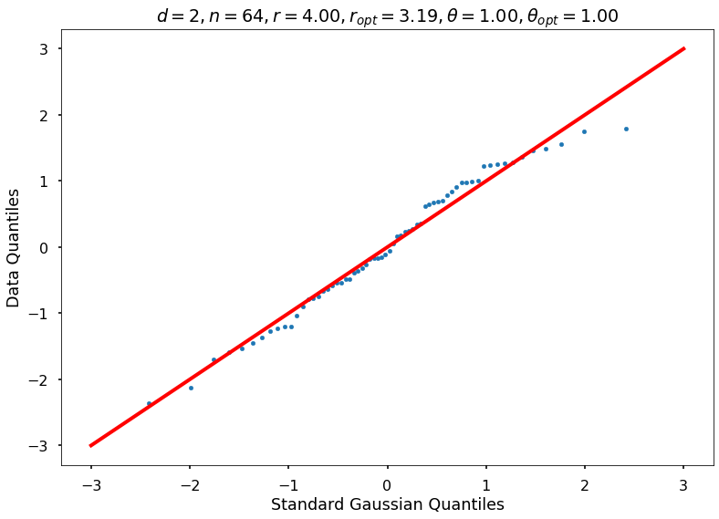
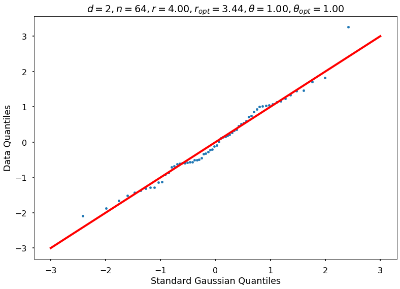
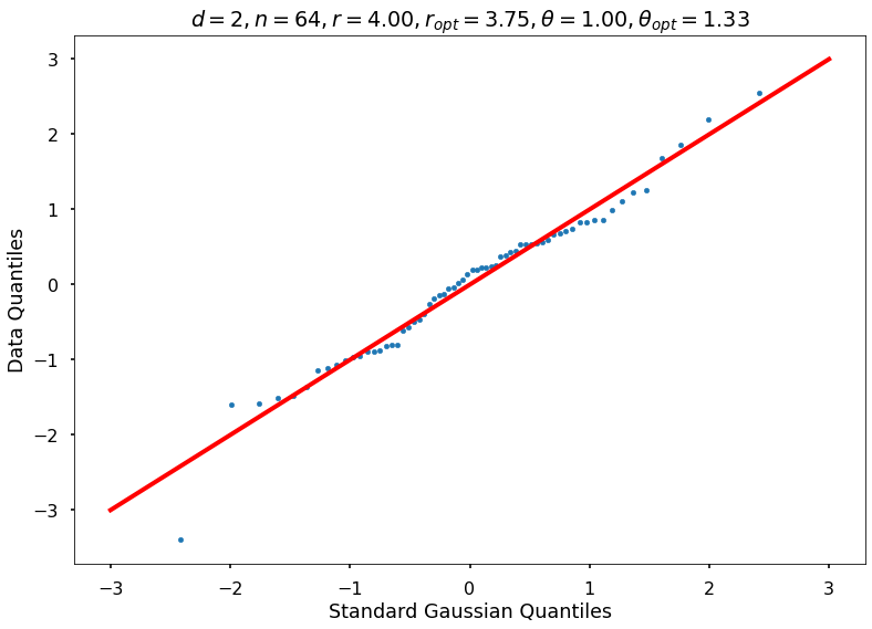
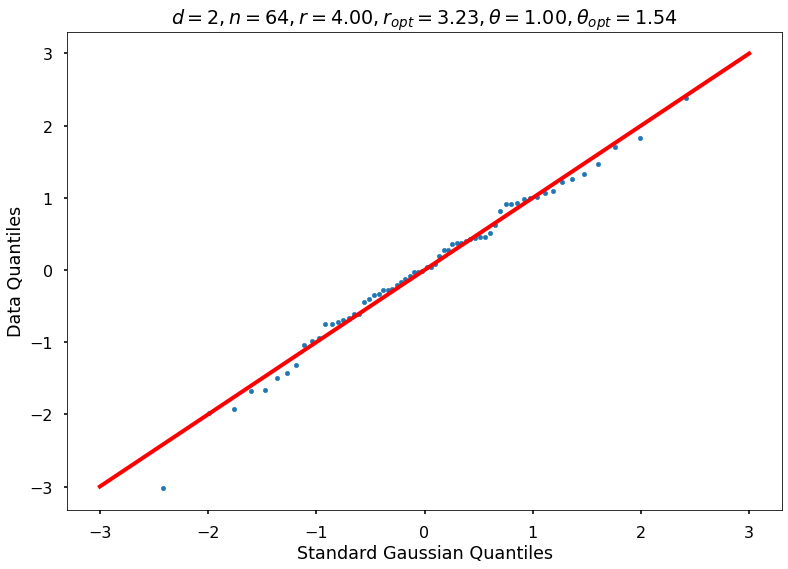
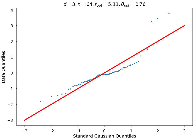
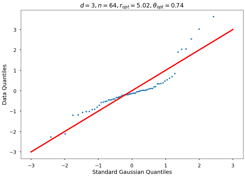
Utility function to draw qqplot or normplot

def create_quant_plot(type, vz_real, fName, dim, iii, r, rOpt, theta, thetaOpt):
    hFigNormplot, axFigNormplot = plt.subplots()

    n = len(vz_real)
    if type == 'normplot':
        axFigNormplot.normplot(vz_real)
    else:
        q = (np.arange(1, n + 1) - 1 / 2) / n
        stNorm = gaussnorm.ppf(q)  # norminv: quantiles of standard normal
        axFigNormplot.scatter(stNorm, sorted(vz_real), s=20)  # marker='.',
        axFigNormplot.plot([-3, 3], [-3, 3], marker='_', linewidth=4, color='red')
        axFigNormplot.set_xlabel('Standard Gaussian Quantiles')
        axFigNormplot.set_ylabel('Data Quantiles')

    if theta:
        plt_title = f'$d={dim}, n={n}, r={r:1.2f}, r_{{opt}}={rOpt:1.2f}, \\theta={theta:1.2f}, \\theta_{{opt}}={thetaOpt:1.2f}$'
        plt_filename = f'{fName}-QQPlot_n-{n}_d-{dim}_r-{r * 100}_th-{100 * theta}_case-{iii}.jpg'
    else:
        plt_title = f'$d={dim}, n={n}, r_{{opt}}={rOpt:1.2f}, \\theta_{{opt}}={thetaOpt:1.2f}$'
        plt_filename = f'{fName}-QQPlot_n-{n}_d-{dim}_case-{iii}.jpg'

    axFigNormplot.set_title(plt_title)
    hFigNormplot.savefig(plt_filename)

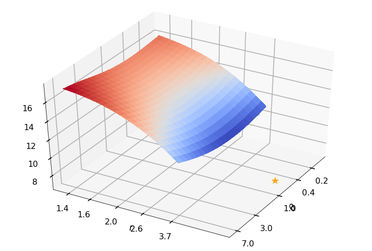
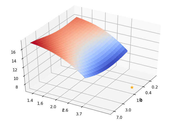
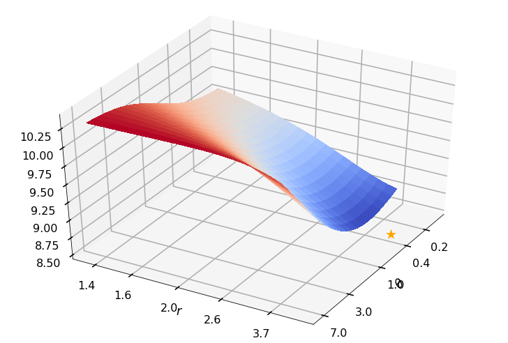
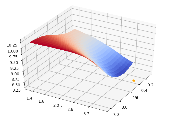
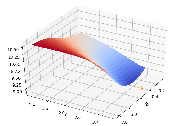
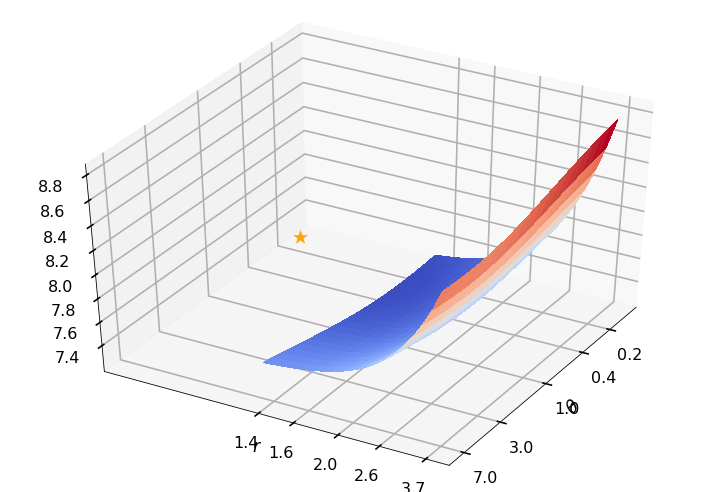
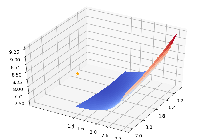
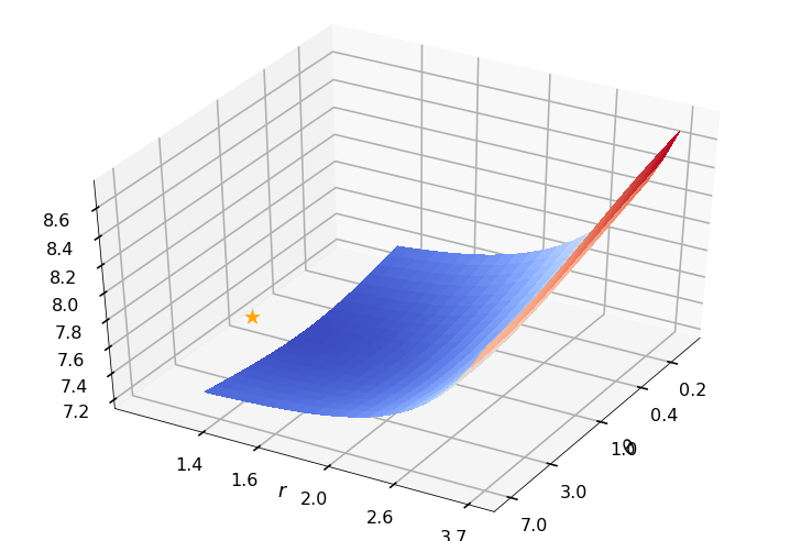
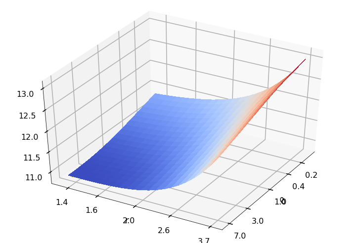
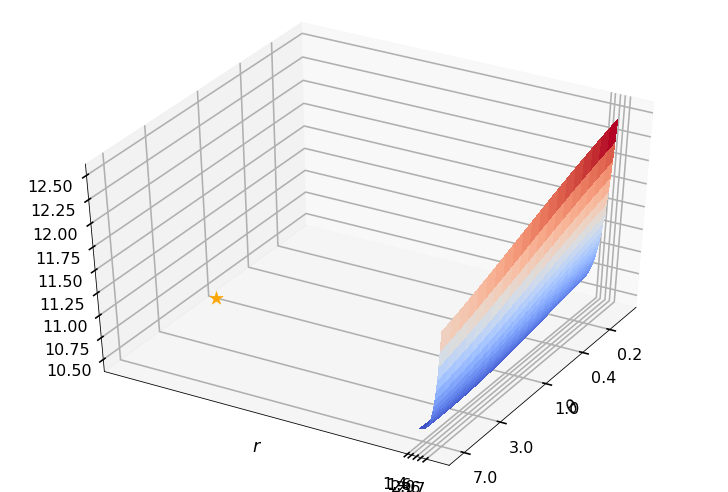
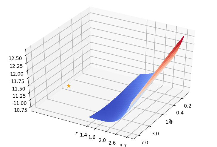
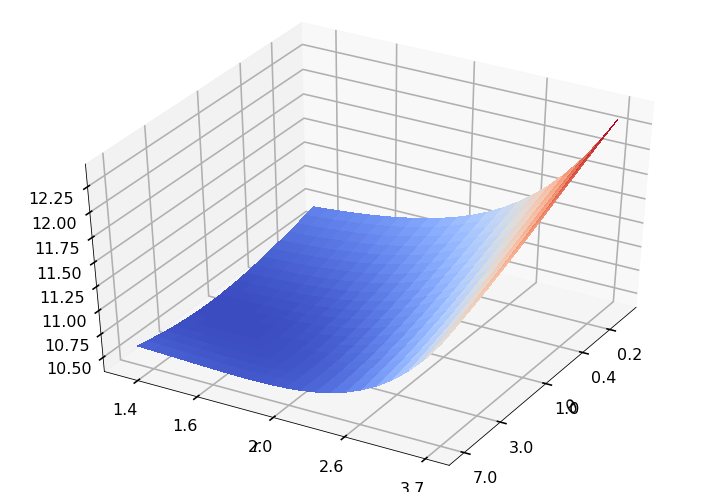
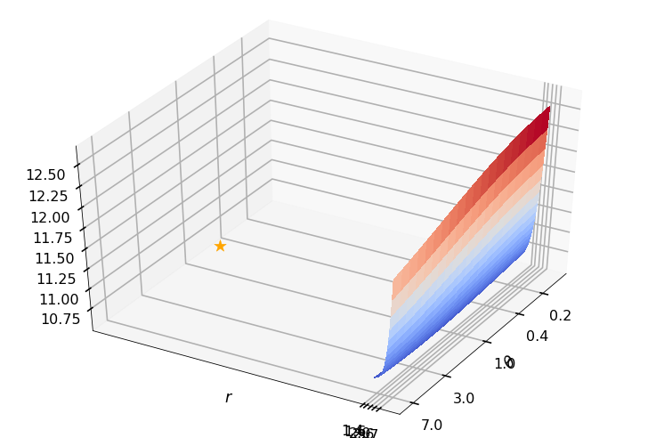
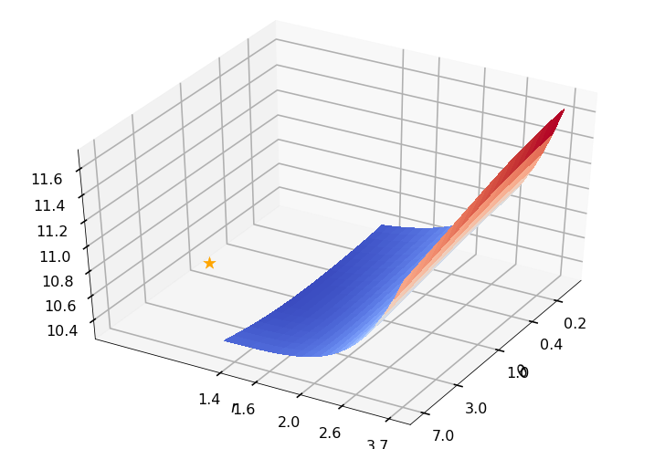
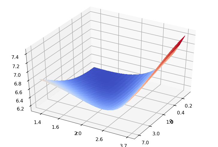
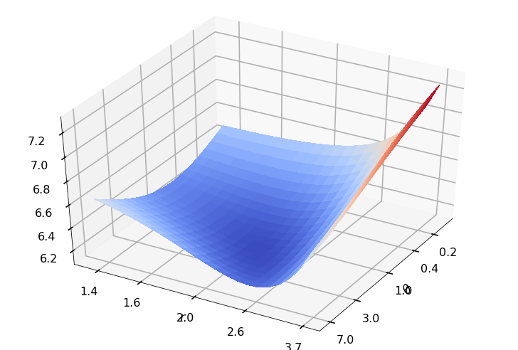
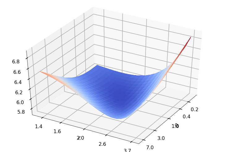
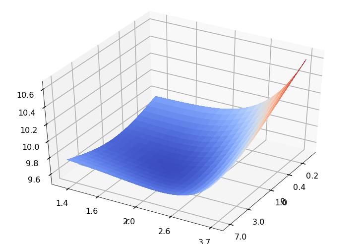
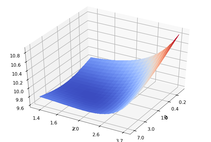
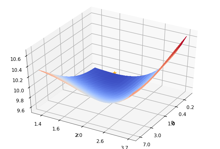
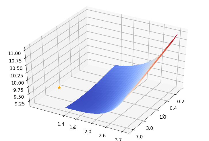
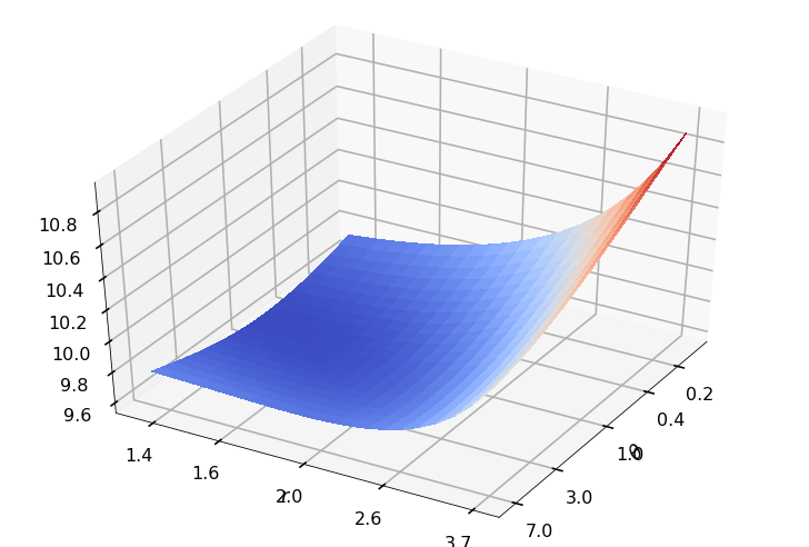
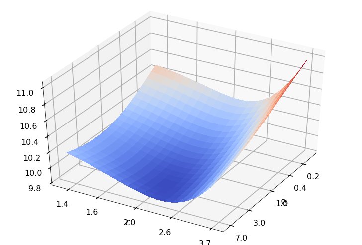
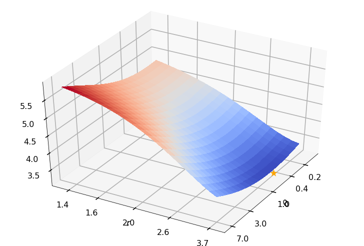
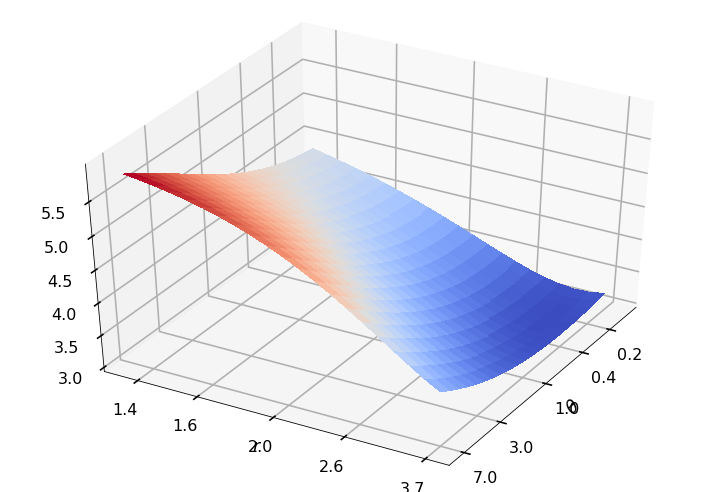
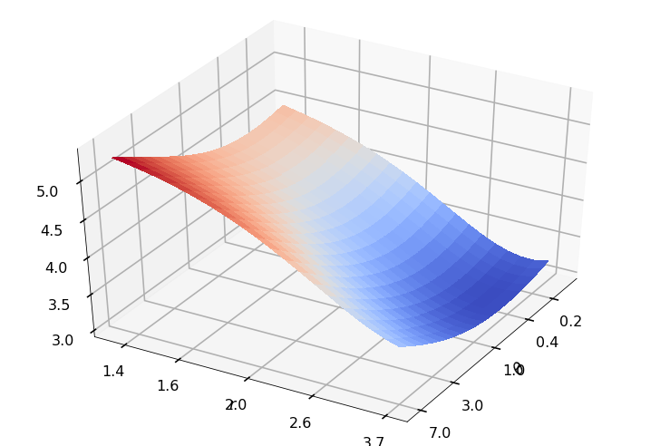
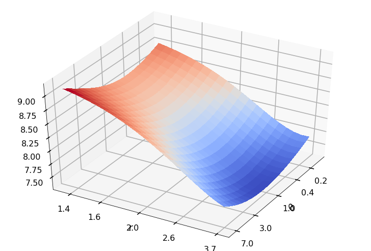
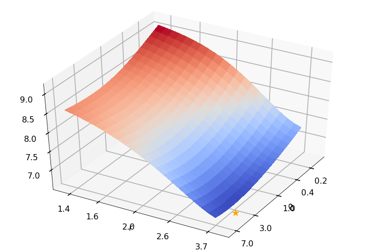
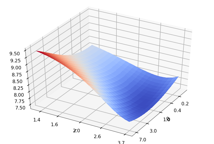
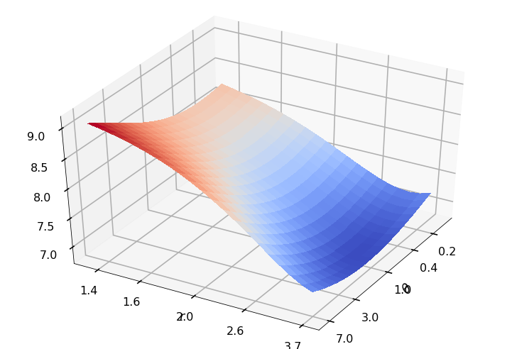
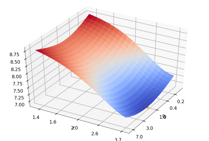
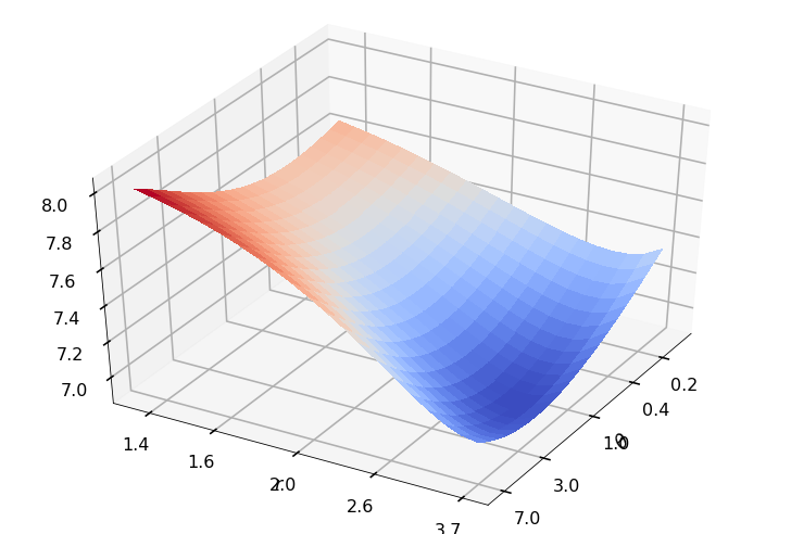
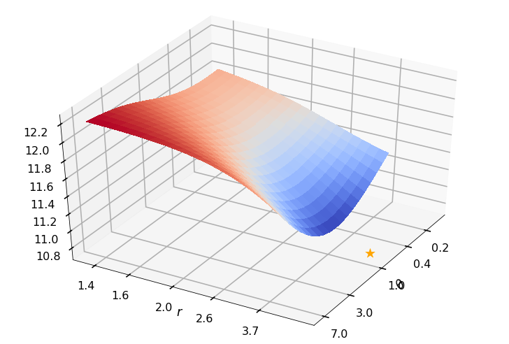
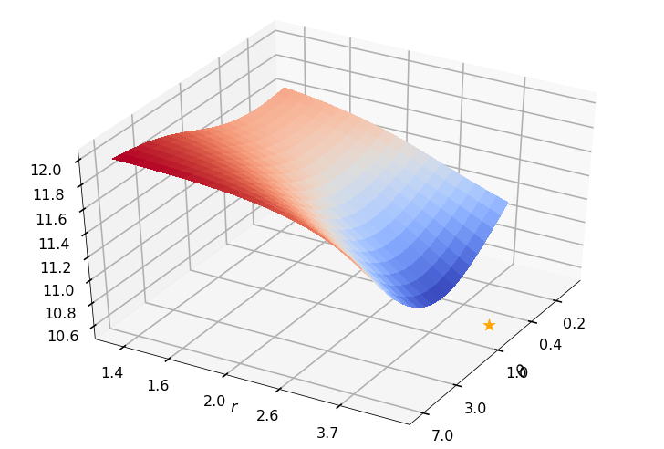
Utility function to plot the objective function and minimum

def create_surf_plot(fName, lnthth, lnordord, objfun, objobj, lnParamsOpt, r, theta, iii):
    figH, axH = plt.subplots(subplot_kw={"projection": "3d"})
    axH.view_init(40, 30)
    shandle = axH.plot_surface(lnthth, lnordord, objobj, cmap=cm.coolwarm,
                               linewidth=0, antialiased=False, alpha=0.8)
    xt = np.array([.2, 0.4, 1, 3, 7])
    axH.set_xticks(np.log(xt))
    axH.set_xticklabels(xt.astype(str))
    yt = np.array([1.4, 1.6, 2, 2.6, 3.7])
    axH.set_yticks(np.log(yt - 1))
    axH.set_yticklabels(yt.astype(str))
    axH.set_xlabel('$\\theta$')
    axH.set_ylabel('$r$')

    axH.scatter(lnParamsOpt[0], lnParamsOpt[1], objfun(lnParamsOpt) * 1.002,
                s=200, color='orange', marker='*', alpha=0.8)
    if theta:
        filename = f'{fName}-ObjFun_n-{npts}_d-{dim}_r-{r * 100}_th-{100 * theta}_case-{iii}.jpg'
    else:
        filename = f'{fName}-ObjFun_n-{npts}_d-{dim}_case-{iii}.jpg'
    figH.savefig(filename)

Minimum working example to demonstrate Gaussian diagnostics concept

def gaussian_diagnostics_engine(whEx, dim, npts, r, fpar, nReps, nPlots):
    whEx = whEx - 1
    fNames = ['ExpCos', 'Keister', 'rand']
    ptransforms = ['none', 'C1sin', 'none']
    fName = fNames[whEx]
    ptransform = ptransforms[whEx]

    rOptAll = [0]*nRep
    thOptAll = [0]*nRep

    # parameters for random function
    # seed = 202326
    if whEx == 2:
        rfun = r / 2
        f_mean = fpar[2]
        f_std_a = fpar[0]  # this is square root of the a in the talk
        f_std_b = fpar[1]  # this is square root of the b in the talk
        theta = (f_std_a / f_std_b) ** 2
    else:
        theta = None

    for iii in range(nReps):
        seed = np.random.randint(low=1, high=1e6)  # different each rep
        shift = np.random.rand(1, dim)

        distribution = Lattice(dimension=dim, order='linear')
        xpts, xlat = distribution.gen_samples(n_min=0, n_max=npts, warn=False, return_unrandomized=True)

        if fName == 'ExpCos':
            integrand = lambda x: np.exp(np.sum(np.cos(2 * np.pi * x), axis=1))
        elif fName == 'Keister':
            keister = Keister(Lattice(dimension=dim, order='linear'))
            integrand = lambda x: keister.f(x)
        elif fName == 'rand':
            integrand = lambda x: f_rand(x, rfun, f_std_a, f_std_b, f_mean, seed)
        else:
            print('Invalid function name')
            return

        y = doPeriodTx(xpts, integrand, ptransform)

        ftilde = np.fft.fft(y)  # fourier coefficients
        ftilde[0] = 0  # ftilde = \mV**H(\vf - m \vone), subtract mean
        if dim == 1:
            hFigIntegrand = plt.figure()
            plt.scatter(xpts, y, 10)
            plt.title(f'{fName}_n-{npts}_Tx-{ptransform}')
            hFigIntegrand.savefig(f'{fName}_n-{npts}_Tx-{ptransform}_rFun-{rfun:1.2f}.png')

        def objfun(lnParams):
            loss, Lambda, RKHSnorm = ObjectiveFunction(np.exp(lnParams[0]), 1 + np.exp(lnParams[1]), xlat, ftilde)
            return loss

        ## Plot the objective function
        lnthetarange = np.arange(-2, 2.2, 0.2)  # range of log(theta) for plotting
        lnorderrange = np.arange(-1, 1.1, 0.1)  # range of log(r) for plotting
        [lnthth, lnordord] = np.meshgrid(lnthetarange, lnorderrange)
        objobj = np.zeros(lnthth.shape)
        for ii in range(lnthth.shape[0]):
            for jj in range(lnthth.shape[1]):
                objobj[ii, jj] = objfun([lnthth[ii, jj], lnordord[ii, jj]])

        objMinAppx, which = objobj.min(), objobj.argmin()
        # [whichrow, whichcol] = ind2sub(lnthth.shape, which)
        [whichrow, whichcol] = np.unravel_index(which, lnthth.shape)
        lnthOptAppx = lnthth[whichrow, whichcol]
        thetaOptAppx = np.exp(lnthOptAppx)
        lnordOptAppx = lnordord[whichrow, whichcol]
        orderOptAppx = 1 + np.exp(lnordOptAppx)
        # print(objMinAppx)  # minimum objective function by brute force search

        ## Optimize the objective function
        result = fminsearch(objfun, x0=[lnthOptAppx, lnordOptAppx], xtol=1e-3, full_output=True, disp=False)
        lnParamsOpt, objMin = result[0], result[1]
        # print(objMin)  # minimum objective function by Nelder-Mead
        thetaOpt = np.exp(lnParamsOpt[0])
        rOpt = 1 + np.exp(lnParamsOpt[1])
        rOptAll[iii] = rOpt
        thOptAll[iii] = thetaOpt
        print(f'{iii}: thetaOptAppx={thetaOptAppx:7.5f}, rOptAppx={orderOptAppx:7.5f}, '
              f'objMinAppx={objMinAppx:7.5f}, objMin={objMin:7.5f}')

        if iii <= nPlots:
            create_surf_plot(fName, lnthth, lnordord, objfun, objobj, lnParamsOpt, r, theta, iii)

        vlambda = kernel2(thetaOpt, rOpt, xlat)
        s2 = sum(abs(ftilde[2:] ** 2) / vlambda[2:]) / (npts ** 2)
        vlambda = s2 * vlambda

        # apply transform
        # $\vZ = \frac 1n \mV \mLambda**{-\frac 12} \mV**H(\vf - m \vone)$
        # np.fft also includes 1/n division
        vz = np.fft.ifft(ftilde / np.sqrt(vlambda))
        vz_real = np.real(vz)  # vz must be real as intended by the transformation

        if iii <= nPlots:
            create_quant_plot('qqplot', vz_real, fName, dim, iii, r, rOpt, theta, thetaOpt)

        r_str = f"{r: 7.5f}" if type(r) == float else str(r)
        theta_str = f"{theta: 7.5f}" if type(theta) == float else str(theta)
        print(f'\t r = {r_str}, rOpt = {rOpt:7.5f}, theta = {theta_str}, thetaOpt = {thetaOpt:7.5f}\n')

    return [theta, rOptAll, thOptAll, fName]

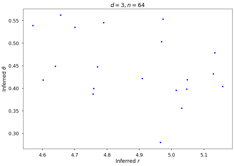
Example 1: Exponential of Cosine

fwh = 1
dim = 3
npts = 2 ** 6
nRep = 20
nPlot = 2
[_, rOptAll, thOptAll, fName] = \
    gaussian_diagnostics_engine(fwh, dim, npts, None, None, nRep, nPlot)

## Plot Exponential Cosine example
figH = plt.figure()
plt.scatter(rOptAll, thOptAll, s=20, color='blue')
# axis([4 6 0.1 10])
# set(gca,'yscale','log')
plt.title(f'$d = {dim}, n = {npts}$')
plt.xlabel('Inferred $r$')
plt.ylabel('Inferred $\\theta$')
# print(f'{fName}-rthInfer-n-{npts}-d-{dim}')
figH.savefig(f'{fName}-rthInfer-n-{npts}-d-{dim}.jpg')

0: thetaOptAppx=0.36788, rOptAppx=3.71828, objMinAppx=8.62452, objMin=8.55148
     r = None, rOpt = 4.60174, theta = None, thetaOpt = 0.41845

1: thetaOptAppx=0.36788, rOptAppx=3.71828, objMinAppx=8.45167, objMin=8.30125
     r = None, rOpt = 5.04805, theta = None, thetaOpt = 0.41943

2: thetaOptAppx=0.44933, rOptAppx=3.71828, objMinAppx=8.94756, objMin=8.86498
     r = None, rOpt = 4.70102, theta = None, thetaOpt = 0.53527

3: thetaOptAppx=0.36788, rOptAppx=3.71828, objMinAppx=8.44618, objMin=8.29799
     r = None, rOpt = 5.04699, theta = None, thetaOpt = 0.39835

4: thetaOptAppx=0.36788, rOptAppx=3.71828, objMinAppx=8.45494, objMin=8.28315
     r = None, rOpt = 5.15814, theta = None, thetaOpt = 0.40447

5: thetaOptAppx=0.36788, rOptAppx=3.71828, objMinAppx=8.57968, objMin=8.47859
     r = None, rOpt = 4.75680, theta = None, thetaOpt = 0.38761

6: thetaOptAppx=0.36788, rOptAppx=3.71828, objMinAppx=8.69501, objMin=8.61827
     r = None, rOpt = 4.63978, theta = None, thetaOpt = 0.44889

7: thetaOptAppx=0.44933, rOptAppx=3.71828, objMinAppx=9.00638, objMin=8.91494
     r = None, rOpt = 4.78933, theta = None, thetaOpt = 0.54575

8: thetaOptAppx=0.44933, rOptAppx=3.71828, objMinAppx=9.01994, objMin=8.90784
     r = None, rOpt = 4.97296, theta = None, thetaOpt = 0.55376

9: thetaOptAppx=0.44933, rOptAppx=3.71828, objMinAppx=8.79716, objMin=8.67140
     r = None, rOpt = 4.96866, theta = None, thetaOpt = 0.50381

10: thetaOptAppx=0.36788, rOptAppx=3.71828, objMinAppx=8.79790, objMin=8.65545
     r = None, rOpt = 5.13328, theta = None, thetaOpt = 0.47860

11: thetaOptAppx=0.36788, rOptAppx=3.71828, objMinAppx=8.47457, objMin=8.34622
     r = None, rOpt = 4.90876, theta = None, thetaOpt = 0.42187

12: thetaOptAppx=0.36788, rOptAppx=3.71828, objMinAppx=8.49223, objMin=8.39115
     r = None, rOpt = 4.75830, theta = None, thetaOpt = 0.39949

13: thetaOptAppx=0.36788, rOptAppx=3.71828, objMinAppx=8.61363, objMin=8.51504
     r = None, rOpt = 4.77039, theta = None, thetaOpt = 0.44782

14: thetaOptAppx=0.30119, rOptAppx=3.71828, objMinAppx=8.48461, objMin=8.34370
     r = None, rOpt = 5.03099, theta = None, thetaOpt = 0.35658

15: thetaOptAppx=0.44933, rOptAppx=3.71828, objMinAppx=9.03541, objMin=8.96192
     r = None, rOpt = 4.65646, theta = None, thetaOpt = 0.56225

16: thetaOptAppx=0.30119, rOptAppx=3.71828, objMinAppx=8.24322, objMin=8.08881
     r = None, rOpt = 4.96519, theta = None, thetaOpt = 0.28016

17: thetaOptAppx=0.36788, rOptAppx=3.71828, objMinAppx=8.53428, objMin=8.37148
     r = None, rOpt = 5.12928, theta = None, thetaOpt = 0.43230

18: thetaOptAppx=0.44933, rOptAppx=3.71828, objMinAppx=8.95320, objMin=8.88930
     r = None, rOpt = 4.57031, theta = None, thetaOpt = 0.53913

19: thetaOptAppx=0.30119, rOptAppx=3.71828, objMinAppx=8.42682, objMin=8.27037
     r = None, rOpt = 5.01433, theta = None, thetaOpt = 0.39608

# close all the previous plots to freeup memory
plt.close('all')

Example 2: Random function

## Tests with random function
rArray = [1.5, 2, 4]
nrArr = len(rArray)
fParArray = [[0.5, 1, 2], [1, 1, 1], [1, 1, 1]]
nfPArr = len(fParArray)
fwh = 3
dim = 2
npts = 2 ** 6
nRep = 5  # reduced from 20 to reduce the plots
nPlot = 2
thetaAll = np.zeros((nrArr, nfPArr))
rOptAll = np.zeros((nrArr, nfPArr, nRep))
thOptAll = np.zeros((nrArr, nfPArr, nRep))
for jjj in range(nrArr):
    for kkk in range(nfPArr):
        thetaAll[jjj, kkk], rOptAll[jjj, kkk, :], thOptAll[jjj, kkk, :], fName = \
            gaussian_diagnostics_engine(fwh, dim, npts, rArray[jjj], fParArray[kkk], nRep, nPlot)

7.287181247404372
7.268099510403598
r =  1.50000, rOpt = 1.08321, theta =  0.25000, thetaOpt = 0.18959

7.439206667642468
7.420522178757865
r =  1.50000, rOpt = 1.08048, theta =  0.25000, thetaOpt = 0.37974

7.237565543945999
7.2348776269121124
r =  1.50000, rOpt = 1.24698, theta =  0.25000, thetaOpt = 1.00000

7.144410538581832
7.143842961246502
r =  1.50000, rOpt = 1.75370, theta =  0.25000, thetaOpt = 2.48385

7.317407633559816
7.317303232422838
r =  1.50000, rOpt = 1.55240, theta =  0.25000, thetaOpt = 0.64486

10.864589626523202
10.864398926256648
r =  1.50000, rOpt = 1.38658, theta =  1.00000, thetaOpt = 6.87095

10.506347397179722
10.483539417962092
r =  1.50000, rOpt = 1.00000, theta =  1.00000, thetaOpt = 1.32199

10.732206996328214
10.7195206863197
r =  1.50000, rOpt = 1.03409, theta =  1.00000, thetaOpt = 0.96591

10.713950538487756
10.706754036079342
r =  1.50000, rOpt = 1.70351, theta =  1.00000, thetaOpt = 12.89957

10.3923460325491
10.367674586632736
r =  1.50000, rOpt = 1.00000, theta =  1.00000, thetaOpt = 0.60214

10.481613959193172
10.481573119044445
r =  1.50000, rOpt = 1.44574, theta =  1.00000, thetaOpt = 1.86278

10.624184268139306
10.587513806429946
r =  1.50000, rOpt = 1.00000, theta =  1.00000, thetaOpt = 0.65292

10.336255790040328
10.32105621339534
r =  1.50000, rOpt = 1.11594, theta =  1.00000, thetaOpt = 1.00000

10.699799283646295
10.69967356700936
r =  1.50000, rOpt = 1.44362, theta =  1.00000, thetaOpt = 2.38455

10.51500018761115
10.506939121521446
r =  1.50000, rOpt = 1.17968, theta =  1.00000, thetaOpt = 8.69595

6.158209638152028
6.157963442419079
r = 2, rOpt = 1.57828, theta =  0.25000, thetaOpt = 0.23715

c:toolsminiconda3envsqmcpy1libsite-packagesipykernel_launcher.py:66
    RuntimeWarning: More than 20 figures have been opened. Figures created through the pyplot interface (matplotlib.pyplot.figure) are retained until explicitly closed and may consume too much memory. (To control this warning, see the rcParam figure.max_open_warning).
c:toolsminiconda3envsqmcpy1libsite-packagesipykernel_launcher.py:2
    RuntimeWarning: More than 20 figures have been opened. Figures created through the pyplot interface (matplotlib.pyplot.figure) are retained until explicitly closed and may consume too much memory. (To control this warning, see the rcParam figure.max_open_warning).

6.157143147450321
6.156543364291681
r = 2, rOpt = 2.15114, theta =  0.25000, thetaOpt = 2.01164

5.75085055457758
5.750809973133201
r = 2, rOpt = 2.00000, theta =  0.25000, thetaOpt = 0.68772

6.069632328951123
6.069055139303397
r = 2, rOpt = 1.84615, theta =  0.25000, thetaOpt = 0.42398

6.034985224985181
6.034874930815441
r = 2, rOpt = 1.67831, theta =  0.25000, thetaOpt = 0.53403

9.551558949940272
9.551384972239866
r = 2, rOpt = 1.92009, theta =  1.00000, thetaOpt = 1.58611

9.633085074190632
9.632776824536194
r = 2, rOpt = 1.76012, theta =  1.00000, thetaOpt = 1.73525

9.568557894047606
9.568348412892643
r = 2, rOpt = 1.58769, theta =  1.00000, thetaOpt = 0.13924

9.541751585509552
9.541667509495124
r = 2, rOpt = 1.48197, theta =  1.00000, thetaOpt = 1.41333

9.5396175595642
9.539398408753463
r = 2, rOpt = 1.55887, theta =  1.00000, thetaOpt = 0.12623

9.170505000843896
9.162768712949173
r = 2, rOpt = 1.15246, theta =  1.00000, thetaOpt = 1.68521

9.6238915085669
9.62377543126308
r = 2, rOpt = 1.39439, theta =  1.00000, thetaOpt = 0.86724

9.851657112032425
9.850539894156423
r = 2, rOpt = 2.15206, theta =  1.00000, thetaOpt = 3.90645

9.806190014351044
9.805541561888338
r = 2, rOpt = 2.44945, theta =  1.00000, thetaOpt = 2.23506

9.79209159625104
9.791515852224858
r = 2, rOpt = 1.85087, theta =  1.00000, thetaOpt = 1.61353

3.2161538975858517
3.211437887705981
r = 4, rOpt = 3.84952, theta =  0.25000, thetaOpt = 0.56819

3.1312343157485762
3.1292745389997414
r = 4, rOpt = 3.37450, theta =  0.25000, thetaOpt = 0.30053

3.0695614957742343
3.0682627340993567
r = 4, rOpt = 3.39840, theta =  0.25000, thetaOpt = 0.41193

3.027380943889609
3.0266075283943112
r = 4, rOpt = 3.76590, theta =  0.25000, thetaOpt = 0.36430

3.5228968345657194
3.5143715614313487
r = 4, rOpt = 3.89398, theta =  0.25000, thetaOpt = 0.48767

7.379762232781738
7.376813143468294
r = 4, rOpt = 3.60031, theta =  1.00000, thetaOpt = 1.14533

6.641928348506947
6.617895389661783
r = 4, rOpt = 4.05057, theta =  1.00000, thetaOpt = 4.39747

7.476855960512737
7.476496711605328
r = 4, rOpt = 3.18967, theta =  1.00000, thetaOpt = 1.00000

6.905066745166625
6.731884736747105
r = 4, rOpt = 4.55762, theta =  1.00000, thetaOpt = 2.69082

6.998288530030136
6.956313755828155
r = 4, rOpt = 4.25120, theta =  1.00000, thetaOpt = 1.18999

6.863019673493637
6.8628173704594655
r = 4, rOpt = 3.43551, theta =  1.00000, thetaOpt = 1.00000

6.942054984148132
6.9414476082169205
r = 4, rOpt = 3.74774, theta =  1.00000, thetaOpt = 1.32587

6.928869540278924
6.928780381246793
r = 4, rOpt = 3.23388, theta =  1.00000, thetaOpt = 1.54465

6.864061134245936
6.84621776419379
r = 4, rOpt = 3.98079, theta =  1.00000, thetaOpt = 1.00000

7.027153534225495
6.917713557698754
r = 4, rOpt = 4.51165, theta =  1.00000, thetaOpt = 2.35318

# close all the previous plots to freeup memory
plt.close('all')

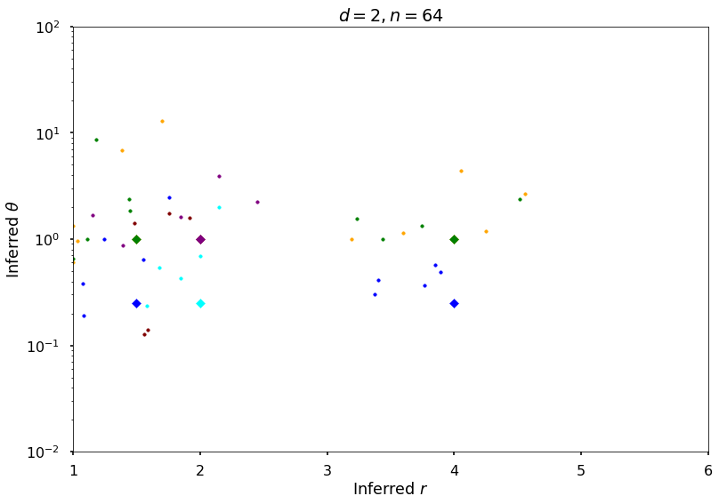
Plot additional figures for random function

figH, axH = plt.subplots()
colorArray = ['blue', 'orange', 'green', 'cyan', 'maroon', 'purple']
nColArray = len(colorArray)
for jjj in range(nrArr):
    for kkk in range(nfPArr):
        clrInd = np.mod(nfPArr * (jjj) + kkk, nColArray)
        clr = colorArray[clrInd]
        axH.scatter(rOptAll[jjj, kkk, :].reshape((nRep, 1)), thOptAll[jjj, kkk, :].reshape((nRep, 1)),
                 s=50, c=clr, marker='.')
        axH.scatter(rArray[jjj], thetaAll[jjj, kkk], s=50, c=clr, marker='D')

axH.set(xlim=[1, 6], ylim=[0.01, 100])
axH.set_yscale('log')
axH.set_title(f'$d = {dim}, n = {npts}$')
axH.set_xlabel('Inferred $r$')
axH.set_ylabel('Inferred $\\theta$')
figH.savefig(f'{fName}-rthInfer-n-{npts}-d-{dim}.jpg')

# close all the previous plots to freeup memory
plt.close('all')

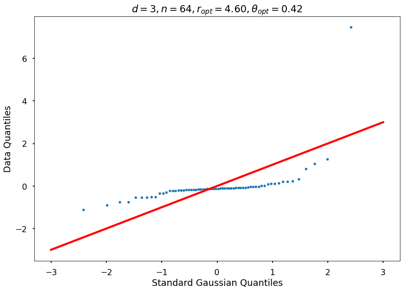
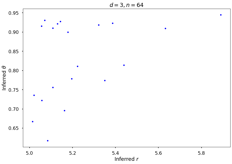
Example 3a: Keister integrand: npts = 64

## Keister example
fwh = 2
dim = 3
npts = 2 ** 6
nRep = 20
nPlot = 2
_, rOptAll, thOptAll, fName = gaussian_diagnostics_engine(fwh, dim, npts, None, None, nRep, nPlot)

## Plot Keister example
figH = plt.figure()
plt.scatter(rOptAll, thOptAll, s=20, color='blue')
# axis([4 6 0.5 1.5])
# set(gca,'yscale','log')
plt.xlabel('Inferred $r$')
plt.ylabel('Inferred $\\theta$')
plt.title(f'$d = {dim}, n = {npts}$')
figH.savefig(f'{fName}-rthInfer-n-{npts}-d-{dim}.jpg')

10.918373367804714
10.74245342720698
r = None, rOpt = 5.17845, theta = None, thetaOpt = 0.90000

10.717466826946536
10.562731448359418
r = None, rOpt = 5.10797, theta = None, thetaOpt = 0.75631

10.688455595826237
10.539160528442594
r = None, rOpt = 5.02081, theta = None, thetaOpt = 0.73583

10.874548555226458
10.610842354541466
r = None, rOpt = 5.63220, theta = None, thetaOpt = 0.90923

10.740805174948838
10.557754768898818
r = None, rOpt = 5.19574, theta = None, thetaOpt = 0.77893

10.928140146153147
10.720109505682482
r = None, rOpt = 5.43883, theta = None, thetaOpt = 0.81368

10.936776084649589
10.748392943135848
r = None, rOpt = 5.32207, theta = None, thetaOpt = 0.91872

10.866161104206988
10.690655913547836
r = None, rOpt = 5.14400, theta = None, thetaOpt = 0.92759

10.613489865692868
10.45889197376518
r = None, rOpt = 5.08381, theta = None, thetaOpt = 0.61740

10.636181168972138
10.467815857368016
r = None, rOpt = 5.16286, theta = None, thetaOpt = 0.69577

10.728895335365538
10.585065856399083
r = None, rOpt = 5.05675, theta = None, thetaOpt = 0.72234

11.031579085996949
10.889786816011357
r = None, rOpt = 5.05532, theta = None, thetaOpt = 0.91526

10.866073731336623
10.548636876696989
r = None, rOpt = 5.88962, theta = None, thetaOpt = 0.94453

10.898763849532882
10.7428251348116
r = None, rOpt = 5.07111, theta = None, thetaOpt = 0.93066

11.04144749198928
10.892511325588508
r = None, rOpt = 5.10849, theta = None, thetaOpt = 0.91039

10.771539976900868
10.602263037779617
r = None, rOpt = 5.22262, theta = None, thetaOpt = 0.81070

10.919713159295926
10.703969564045602
r = None, rOpt = 5.38652, theta = None, thetaOpt = 0.92338

10.775915237177964
10.646594662551685
r = None, rOpt = 5.01369, theta = None, thetaOpt = 0.66747

11.02928162756276
10.874074219278276
r = None, rOpt = 5.12990, theta = None, thetaOpt = 0.92172

10.87752870870672
10.685153898271022
r = None, rOpt = 5.34982, theta = None, thetaOpt = 0.77387

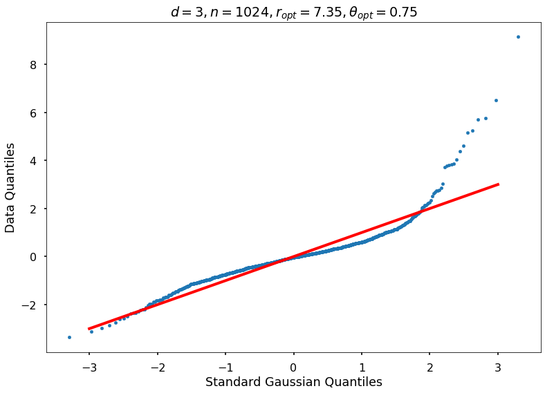
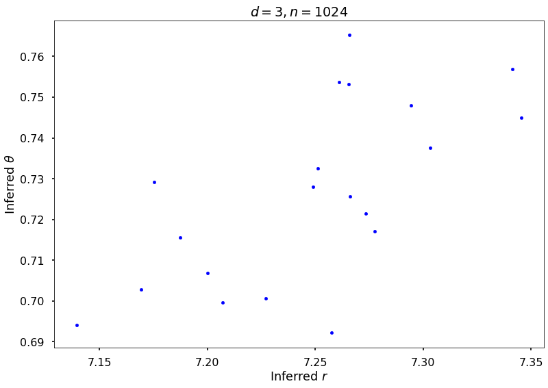
Example 3b: Keister integrand: npts = 1024

## Keister example
fwh = 2
dim = 3
npts = 2 ** 10
nRep = 20
nPlot = 2
_, rOptAll, thOptAll, fName = gaussian_diagnostics_engine(fwh, dim, npts, None, None, nRep, nPlot)

## Plot Keister example
figH = plt.figure()
plt.scatter(rOptAll, thOptAll, s=20, color='blue')
# axis([4 6 0.5 1.5])
# set(gca,'yscale','log')
plt.xlabel('Inferred $r$')
plt.ylabel('Inferred $\\theta$')
plt.title(f'$d = {dim}, n = {npts}$')
figH.savefig(f'{fName}-rthInfer-n-{npts}-d-{dim}.jpg')

10.596244143639485
7.142978946028139
r = None, rOpt = 7.18724, theta = None, thetaOpt = 0.71553

10.594856691086207
7.096409091118618
r = None, rOpt = 7.26586, theta = None, thetaOpt = 0.76520

10.591375134255042
7.0166323209172194
r = None, rOpt = 7.34554, theta = None, thetaOpt = 0.74504

10.595755571171377
7.067858016018031
r = None, rOpt = 7.34121, theta = None, thetaOpt = 0.75696

10.595982354998483
7.1228385587643395
r = None, rOpt = 7.22718, theta = None, thetaOpt = 0.70060

10.596298140666004
7.104717917027118
r = None, rOpt = 7.27766, theta = None, thetaOpt = 0.71703

10.592187612685716
7.0859774608781745
r = None, rOpt = 7.26092, theta = None, thetaOpt = 0.75369

10.596120527059021
7.10600296848717
r = None, rOpt = 7.25766, theta = None, thetaOpt = 0.69220

10.594256056513693
7.105374164104877
r = None, rOpt = 7.25124, theta = None, thetaOpt = 0.73247

10.596614398709978
7.137622143665308
r = None, rOpt = 7.20010, theta = None, thetaOpt = 0.70688

10.598230772383527
7.186852606944651
r = None, rOpt = 7.13933, theta = None, thetaOpt = 0.69409

10.597856894192905
7.126442092925792
r = None, rOpt = 7.27342, theta = None, thetaOpt = 0.72154

10.595526689101934
7.101590379268407
r = None, rOpt = 7.26605, theta = None, thetaOpt = 0.72566

10.593990233649055
7.128838039518072
r = None, rOpt = 7.17539, theta = None, thetaOpt = 0.72916

10.594285418816956
7.138947266052696
r = None, rOpt = 7.16931, theta = None, thetaOpt = 0.70287

10.597310034462971
7.117069509729076
r = None, rOpt = 7.30321, theta = None, thetaOpt = 0.73752

10.592677212556865
7.085904146817816
r = None, rOpt = 7.26545, theta = None, thetaOpt = 0.75314

10.592216478157543
7.05396738656259
r = None, rOpt = 7.29427, theta = None, thetaOpt = 0.74802

10.59392746212006
7.109982966182546
r = None, rOpt = 7.20702, theta = None, thetaOpt = 0.69972

10.595997284727325
7.111744447354244
r = None, rOpt = 7.24907, theta = None, thetaOpt = 0.72795