Purdue University Colloquim Talk
Computations and Figures for Department of Statistics Colloquim at Purdue University
presented on Friday, March 3, 2023, slides here
Import the necessary packages and set up plotting routines
import matplotlib.pyplot as plt
import numpy as np
import qmcpy as qp
import time  #timing routines
import warnings  #to suppress warnings when needed
import pickle  #write output to a file and load it back in
from copy import deepcopy

plt.rc('font', size=16)  #set defaults so that the plots are readable
plt.rc('axes', titlesize=16)
plt.rc('axes', labelsize=16)
plt.rc('xtick', labelsize=16)
plt.rc('ytick', labelsize=16)
plt.rc('legend', fontsize=16)
plt.rc('figure', titlesize=16)

#a helpful plotting method to show increasing numbers of points
def plot_successive_points(distrib,ld_name,first_n=64,n_cols=1,
                           pt_clr=['tab:blue', 'tab:green', 'k', 'tab:cyan', 'tab:purple', 'tab:orange'],
                           xlim=[0,1],ylim=[0,1]):
  fig,ax = plt.subplots(nrows=1,ncols=n_cols,figsize=(5*n_cols,5.5))
  if n_cols==1: ax = [ax]
  last_n = first_n*(2**n_cols)
  points = distrib.gen_samples(n=last_n)
  for i in range(n_cols):
    n = first_n
    nstart = 0
    for j in range(i+1):
      n = first_n*(2**j)
      ax[i].scatter(points[nstart:n,0],points[nstart:n,1],color=pt_clr[j])
      nstart = n
    ax[i].set_title('n = %d'%n)
    ax[i].set_xlim(xlim); ax[i].set_xticks(xlim); ax[i].set_xlabel('$x_{i,1}$')
    ax[i].set_ylim(ylim); ax[i].set_yticks(ylim); ax[i].set_ylabel('$x_{i,2}$')
    ax[i].set_aspect((xlim[1]-xlim[0])/(ylim[1]-ylim[0]))
  fig.suptitle('%s Points'%ld_name, y=0.87)
  return fig

print('QMCPy Version',qp.__version__)
QMCPy Version 1.3.2
Set the path to save the figures here
figpath = '' #this path sends the figures to the directory that you want
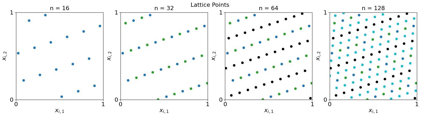
Here are some plots of IID and Low Discrepancy (LD) Points
Lattice points first
d = 5 #dimension
n = 16 #number of points
ld = qp.Lattice(d) #define the generator
xpts = ld.gen_samples(n) #generate points
print(xpts)
fig = plot_successive_points(ld,'Lattice',first_n=n,n_cols=4)
fig.savefig(figpath+'latticepts.eps',format='eps')
[[3.99318970e-01 6.57874778e-01 8.98029521e-01 3.75576673e-01
  8.76944929e-01]
 [8.99318970e-01 1.57874778e-01 3.98029521e-01 8.75576673e-01
  3.76944929e-01]
 [6.49318970e-01 4.07874778e-01 6.48029521e-01 6.25576673e-01
  1.26944929e-01]
 [1.49318970e-01 9.07874778e-01 1.48029521e-01 1.25576673e-01
  6.26944929e-01]
 [5.24318970e-01 3.28747777e-02 2.73029521e-01 5.00576673e-01
  1.94492924e-03]
 [2.43189699e-02 5.32874778e-01 7.73029521e-01 5.76672905e-04
  5.01944929e-01]
 [7.74318970e-01 7.82874778e-01 2.30295212e-02 7.50576673e-01
  2.51944929e-01]
 [2.74318970e-01 2.82874778e-01 5.23029521e-01 2.50576673e-01
  7.51944929e-01]
 [4.61818970e-01 3.45374778e-01 8.55295212e-02 4.38076673e-01
  4.39444929e-01]
 [9.61818970e-01 8.45374778e-01 5.85529521e-01 9.38076673e-01
  9.39444929e-01]
 [7.11818970e-01 9.53747777e-02 8.35529521e-01 6.88076673e-01
  6.89444929e-01]
 [2.11818970e-01 5.95374778e-01 3.35529521e-01 1.88076673e-01
  1.89444929e-01]
 [5.86818970e-01 7.20374778e-01 4.60529521e-01 5.63076673e-01
  5.64444929e-01]
 [8.68189699e-02 2.20374778e-01 9.60529521e-01 6.30766729e-02
  6.44449292e-02]
 [8.36818970e-01 4.70374778e-01 2.10529521e-01 8.13076673e-01
  8.14444929e-01]
 [3.36818970e-01 9.70374778e-01 7.10529521e-01 3.13076673e-01
  3.14444929e-01]]
Next Sobol’ points
ld = qp.Sobol(d) #define the generator
xpts_Sobol = ld.gen_samples(n) #generate points
fig = plot_successive_points(ld,'Sobol\'',first_n=n,n_cols=4)
fig.savefig(figpath+'sobolpts.eps',format='eps')
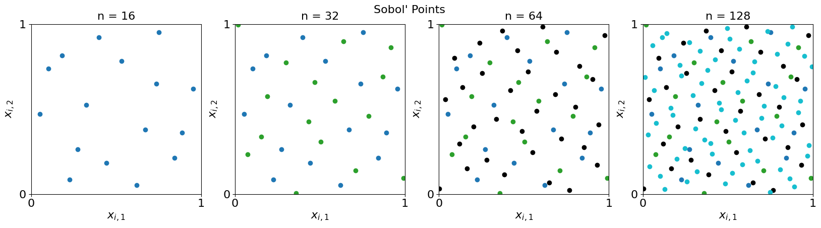
Compare to IID
Note that there are more gaps and clusters
iid = qp.IIDStdUniform(d) #define the generator
xpts = ld.gen_samples(n) #generate points
xpts
fig = plot_successive_points(iid,'IID',first_n=n,n_cols=4)
fig.savefig(figpath+'iidpts.eps',format='eps')

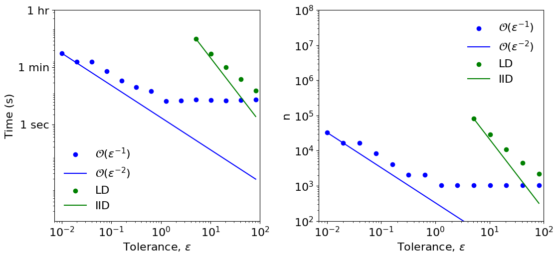
Beam Example Figures
Using computations done below
Plot the time and sample size required to solve for the deflection of the end point using IID and low discrepancy
with open(figpath+'iid_ld.pkl','rb') as myfile: tol_vec,n_tol,ii_iid,ld_time,ld_n,iid_time,iid_n,best_solution_i = pickle.load(myfile)
print(best_solution_i)
fig,ax = plt.subplots(nrows=1,ncols=2,figsize=(13,5.5))
ax[0].scatter(tol_vec[0:n_tol],ld_time[0:n_tol],color='b');
ax[0].plot(tol_vec[0:n_tol],[(ld_time[0]*tol_vec[0])/tol_vec[jj] for jj in range(n_tol)],color='b')
ax[0].scatter(tol_vec[ii_iid:n_tol],iid_time[ii_iid:n_tol],color='g');
ax[0].plot(tol_vec[ii_iid:n_tol],[(iid_time[ii_iid]*(tol_vec[ii_iid]**2))/(tol_vec[jj]**2) for jj in range(ii_iid,n_tol)],color='g')
ax[0].set_ylim([0.001,1000]); ax[0].set_ylabel('Time (s)')
ax[1].scatter(tol_vec[0:n_tol],ld_n[0:n_tol],color='b');
ax[1].plot(tol_vec[0:n_tol],[(ld_n[0]*tol_vec[0])/tol_vec[jj] for jj in range(n_tol)],color='b')
ax[1].scatter(tol_vec[ii_iid:n_tol],iid_n[ii_iid:n_tol],color='g');
ax[1].plot(tol_vec[ii_iid:n_tol],[(iid_n[ii_iid]*(tol_vec[ii_iid]**2))/(tol_vec[jj]**2) for jj in range(ii_iid,n_tol)],color='g')
ax[1].set_ylim([1e2,1e8]); ax[1].set_ylabel('n')
for ii in range(2):
  ax[ii].set_xlim([0.007,100]); ax[ii].set_xlabel('Tolerance, '+r'$\varepsilon$')
  ax[ii].set_xscale('log'); ax[ii].set_yscale('log')
  ax[ii].legend([r'$\mathcal{O}(\varepsilon^{-1})$',r'$\mathcal{O}(\varepsilon^{-2})$','LD','IID'],frameon=False)
  ax[ii].set_aspect(0.65)
ax[0].set_yticks([1, 60, 3600], labels = ['1 sec', '1 min', '1 hr'])
fig.savefig(figpath+'iidldbeam.eps',format='eps',bbox_inches='tight')
[1037.12106673]
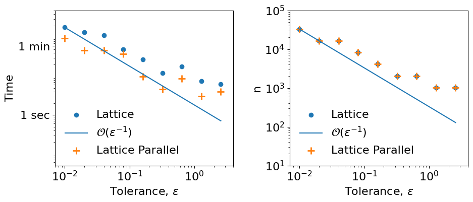
Plot the time and sample size required to solve for the deflection of the whole beam using low discrepancy with and without parallel
with open(figpath+'ld_parallel.pkl','rb') as myfile: tol_vec,n_tol,ld_time,ld_n,ld_p_time,ld_p_n,best_solution = pickle.load(myfile)
print(best_solution_i)
fig,ax = plt.subplots(nrows=1,ncols=2,figsize=(11,4))
ax[0].scatter(tol_vec[0:n_tol],ld_time[0:n_tol],color='tab:blue');
ax[0].plot(tol_vec[0:n_tol],[(ld_time[0]*tol_vec[0])/tol_vec[jj] for jj in range(n_tol)],color='tab:blue')
ax[0].scatter(tol_vec[0:n_tol],ld_p_time[0:n_tol],color='tab:orange',marker = '+',s=100,linewidths=2);
#ax[0].plot(tol_vec[0:n_tol],[(ld_p_time[0]*tol_vec[0])/tol_vec[jj] for jj in range(n_tol)],color='tab:orange')
ax[0].set_ylim([0.05,500]); ax[0].set_ylabel('Time')
ax[1].scatter(tol_vec[0:n_tol],ld_n[0:n_tol],color='tab:blue');
ax[1].plot(tol_vec[0:n_tol],[(ld_n[0]*tol_vec[0])/tol_vec[jj] for jj in range(n_tol)],color='tab:blue')
ax[1].scatter(tol_vec[0:n_tol],ld_p_n[0:n_tol],color='tab:orange',marker = '+',s=100,linewidths=2);
#ax[1].plot(tol_vec[0:n_tol],[(ld_p_n[0]*tol_vec[0])/tol_vec[jj] for jj in range(n_tol)],color='tab:orange')
ax[1].set_ylim([10,1e5]); ax[1].set_ylabel('n')
for ii in range(2):
  ax[ii].set_xlim([0.007,4]); ax[ii].set_xlabel('Tolerance, '+r'$\varepsilon$')
  ax[ii].set_xscale('log'); ax[ii].set_yscale('log')
  ax[ii].legend(['Lattice',r'$\mathcal{O}(\varepsilon^{-1})$','Lattice Parallel',r'$\mathcal{O}(\varepsilon^{-1})$'],frameon=False)
  ax[ii].set_aspect(0.6)
ax[0].set_yticks([1, 60], labels = ['1 sec', '1 min'])
fig.savefig(figpath+'ldparallelbeam.eps',format='eps',bbox_inches='tight')
[1037.12106673]
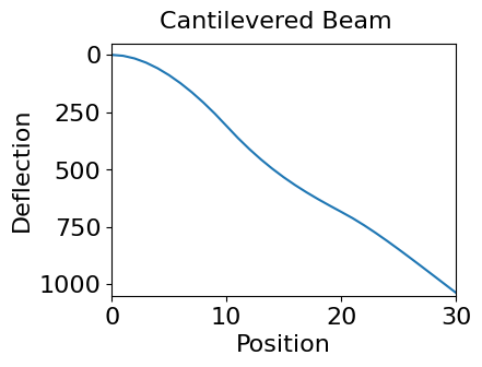
Plot of beam solution
fig,ax = plt.subplots(figsize=(6,3))
ax.plot(best_solution,'-')
ax.set_xlim([0,len(best_solution)-1]); ax.set_xlabel('Position')
ax.set_ylim([1050,-50]);  ax.set_ylabel('Mean Deflection');
ax.set_aspect(0.02)
fig.suptitle('Cantilevered Beam')
fig.savefig(figpath+'cantileveredbeamwords.eps',format='eps',bbox_inches='tight')
qp.util.stop_notebook()
Type 'yes' to continue running notebookyes
Below is long-running code, that we rarely wish to run
Beam Example Computations
Set up the problem using a docker container to solve the ODE
To run this, you need to be running the docker application, https://www.docker.com/products/docker-desktop/
import umbridge #this is the connector
!docker run --name muqbp -d -it -p 4243:4243 linusseelinger/benchmark-muq-beam-propagation:latest #get beam example
d = 3 #dimension of the randomness
lb = 1 #lower bound on randomness
ub = 1.2 #upper bound on randomness
umbridge_config = {"d": d}
model = umbridge.HTTPModel('http://localhost:4243','forward') #this is the original model
outindex = -1 #choose last element of the vector of beam deflections
modeli = deepcopy(model) #and construct a model for just that deflection
modeli.get_output_sizes = lambda *args : [1]
modeli.get_output_sizes()
modeli.__call__ = lambda *args,**kwargs: [[model.__call__(*args,**kwargs)[0][outindex]]]
docker: Error response from daemon: Conflict. The container name "/muqbp" is already in use by container "7f9e0237bd3e72783743efb67f78ce8cc800f5a24835f4191bc423f960cdedac". You have to remove (or rename) that container to be able to reuse that name.
See 'docker run --help'.
First we compute the time required to solve for the deflection of the end point using IID and low discrepancy
ld = qp.Uniform(qp.Lattice(d,seed=7),lower_bound=lb,upper_bound=ub) #lattice points for this problem
ld_integ = qp.UMBridgeWrapper(ld,modeli,umbridge_config,parallel=False) #integrand
iid = qp.Uniform(qp.IIDStdUniform(d),lower_bound=lb,upper_bound=ub) #iid points for this problem
iid_integ = qp.UMBridgeWrapper(iid,modeli,umbridge_config,parallel=False) #integrand
tol = 0.01  #smallest tolerance

n_tol = 14  #number of different tolerances
ii_iid = 9  #make this larger to reduce the time required by not running all cases for IID
tol_vec = [tol*(2**ii) for ii in range(n_tol)]  #initialize vector of tolerances
ld_time = [0]*n_tol; ld_n = [0]*n_tol  #low discrepancy time and number of function values
iid_time = [0]*n_tol; iid_n = [0]*n_tol  #IID time and number of function values
print(f'\nCantilever Beam\n')
print('iteration ', end = '')
for ii in range(n_tol):
  solution, data = qp.CubQMCLatticeG(ld_integ, abs_tol = tol_vec[ii]).integrate()
  if ii == 0:
    best_solution_i = solution
  ld_time[ii] = data.time_integrate
  ld_n[ii] = data.n_total
  if ii >= ii_iid:
    solution, data = qp.CubMCG(iid_integ, abs_tol = tol_vec[ii]).integrate()
    iid_time[ii] = data.time_integrate
    iid_n[ii] = data.n_total
  print(ii, end = ' ')
with open(figpath+'iid_ld.pkl','wb') as myfile:pickle.dump([tol_vec,n_tol,ii_iid,ld_time,ld_n,iid_time,iid_n,best_solution_i],myfile)
Cantilever Beam

iteration 0 1 2 3 4 5 6 7 8 9 10 11 12 13
Next, we compute the time required to solve for the deflection of the whole beam using low discrepancy with and without parallel
ld_integ = qp.UMBridgeWrapper(ld,model,umbridge_config,parallel=False) #integrand
ld_integ_p = qp.UMBridgeWrapper(ld,model,umbridge_config,parallel=8) #integrand with parallel processing

tol = 0.01
n_tol = 9  #number of different tolerances
tol_vec = [tol*(2**ii) for ii in range(n_tol)]  #initialize vector of tolerances
ld_time = [0]*n_tol; ld_n = [0]*n_tol  #low discrepancy time and number of function values
ld_p_time = [0]*n_tol; ld_p_n = [0]*n_tol  #low discrepancy time and number of function values with parallel
print(f'\nCantilever Beam\n')
print('iteration ', end = '')
for ii in range(n_tol):
  solution, data = qp.CubQMCLatticeG(ld_integ, abs_tol = tol_vec[ii]).integrate()
  if ii == 0:
    best_solution = solution
  ld_time[ii] = data.time_integrate
  ld_n[ii] = data.n_total
  solution, data = qp.CubQMCLatticeG(ld_integ_p, abs_tol = tol_vec[ii]).integrate()
  ld_p_time[ii] = data.time_integrate
  ld_p_n[ii] = data.n_total
  print(ii, end = ' ')
with open(figpath+'ld_parallel.pkl','wb') as myfile:pickle.dump([tol_vec,n_tol,ld_time,ld_n,ld_p_time,ld_p_n,best_solution],myfile)
Cantilever Beam

iteration 0 1 2 3 4 5 6 7 8
Shut down docker
!docker rm -f muqbp #shut down docker image
