Integration Examples using QMCPy package

In this demo, we show how to use qmcpy for performing numerical multiple integration of two built-in integrands, namely, the Keister function and the Asian call option payoff. To start, we import the qmcpy module and the function arrange() from numpy for generating evenly spaced discrete vectors in the examples.

from qmcpy import *
from numpy import arange

Keister Example

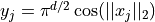
We recall briefly the mathematical definitions of the Keister function, the Gaussian measure, and the Sobol distribution:

Keister integrand: $y_j = \pi^{d/2} \cos(||x_j||_2)$
Gaussian true measure: $\mathcal{N}(0,\frac{1}{2})$
Sobol discrete distribution: $x_j \overset{LD}{\sim} \mathcal{U}(0,1)$

integrand = Keister(Sobol(dimension=3,seed=7))
solution,data = CubQMCSobolG(integrand,abs_tol=.05).integrate()
print(data)

LDTransformData (AccumulateData Object)
    solution        2.170
    comb_bound_low  2.159
    comb_bound_high 2.181
    comb_flags      1
    n_total         2^(10)
    n               2^(10)
    time_integrate  0.002
CubQMCSobolG (StoppingCriterion Object)
    abs_tol         0.050
    rel_tol         0
    n_init          2^(10)
    n_max           2^(35)
Keister (Integrand Object)
Gaussian (TrueMeasure Object)
    mean            0
    covariance      2^(-1)
    decomp_type     PCA
Sobol (DiscreteDistribution Object)
    d               3
    dvec            [0 1 2]
    randomize       LMS_DS
    graycode        0
    entropy         7
    spawn_key       ()

Arithmetic-Mean Asian Put Option: Single Level

In this example, we want to estimate the payoff of an European Asian put option that matures at time $T$ . The key mathematical entities are defined as follows:

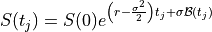
Stock price at time $t_j := jT/d$ for $j=1,\dots,d$ is a function of its initial price $S(0)$ , interest rate $r$ , and volatility $\sigma$ : $S(t_j) = S(0)e^{\left(r-\frac{\sigma^2}{2}\right)t_j + \sigma\mathcal{B}(t_j)}$
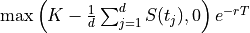
Discounted put option payoff is defined as the difference of a fixed strike price $K$ and the arithmetic average of the underlying stock prices at $d$ discrete time intervals in $[0,T]$ : $\max \left(K-\frac{1}{d}\sum_{j=1}^{d} S(t_j), 0 \right) e^{-rT}$
Brownian motion true measure: $\mathcal{B}(t_j) = \mathcal{B}(t_{j-1}) + Z_j\sqrt{t_j-t_{j-1}} \;$ for $\;Z_j \sim \mathcal{N}(0,1)$
Lattice discrete distribution: $\:\: x_j \overset{LD}{\sim} \mathcal{U}(0,1)$

integrand = AsianOption(
    sampler = IIDStdUniform(dimension=16, seed=7),
    volatility = 0.5,
    start_price = 30,
    strike_price = 25,
    interest_rate = 0.01,
    mean_type = 'arithmetic')
solution,data = CubMCCLT(integrand, abs_tol=.025).integrate()
print(data)

MeanVarData (AccumulateData Object)
    solution        6.257
    error_bound     0.025
    n_total         889904
    n               888880
    levels          1
    time_integrate  1.303
CubMCCLT (StoppingCriterion Object)
    abs_tol         0.025
    rel_tol         0
    n_init          2^(10)
    n_max           10000000000
    inflate         1.200
    alpha           0.010
AsianOption (Integrand Object)
    volatility      2^(-1)
    call_put        call
    start_price     30
    strike_price    25
    interest_rate   0.010
    mean_type       arithmetic
    dim_frac        0
BrownianMotion (TrueMeasure Object)
    time_vec        [0.062 0.125 0.188 ... 0.875 0.938 1.   ]
    drift           0
    mean            [0. 0. 0. ... 0. 0. 0.]
    covariance      [[0.062 0.062 0.062 ... 0.062 0.062 0.062]
                    [0.062 0.125 0.125 ... 0.125 0.125 0.125]
                    [0.062 0.125 0.188 ... 0.188 0.188 0.188]
                    ...
                    [0.062 0.125 0.188 ... 0.875 0.875 0.875]
                    [0.062 0.125 0.188 ... 0.875 0.938 0.938]
                    [0.062 0.125 0.188 ... 0.875 0.938 1.   ]]
    decomp_type     PCA
IIDStdUniform (DiscreteDistribution Object)
    d               2^(4)
    entropy         7
    spawn_key       ()

Arithmetic-Mean Asian Put Option: Multi-Level

This example is similar to the last one except that we use a multi-level method for estimation of the option price. The main idea can be summarized as follows:

$Y_0 = 0$

$Y_1 = \text{ Asian option monitored at } t = [\frac{1}{4}, \frac{1}{2}, \frac{3}{4}, 1]$

$Y_2 = \text{ Asian option monitored at } t= [\frac{1}{16}, \frac{1}{8}, ... , 1]$

$Y_3 = \text{ Asian option monitored at } t= [\frac{1}{64}, \frac{1}{32}, ... , 1]$

$Z_1 = \mathbb{E}[Y_1-Y_0] + \mathbb{E}[Y_2-Y_1] + \mathbb{E}[Y_3-Y_2] = \mathbb{E}[Y_3]$

integrand = AsianOption(
        sampler = IIDStdUniform(seed=7),
        volatility = 0.5,
        start_price = 30,
        strike_price = 25,
        interest_rate = 0.01,
        mean_type = 'arithmetic',
        multilevel_dims = [4,8,16])
solution,data = CubMCCLT(integrand, abs_tol=.025).integrate()
print(data)

MeanVarData (AccumulateData Object)
    solution        6.264
    error_bound     0.025
    n_total         1938085
    n               [1875751.   31235.   28027.]
    levels          3
    time_integrate  0.879
CubMCCLT (StoppingCriterion Object)
    abs_tol         0.025
    rel_tol         0
    n_init          2^(10)
    n_max           10000000000
    inflate         1.200
    alpha           0.010
AsianOption (Integrand Object)
    volatility      2^(-1)
    call_put        call
    start_price     30
    strike_price    25
    interest_rate   0.010
    mean_type       arithmetic
    multilevel_dims [ 4  8 16]
BrownianMotion (TrueMeasure Object)
    time_vec        1
    drift           0
    mean            0
    covariance      1
    decomp_type     PCA
IIDStdUniform (DiscreteDistribution Object)
    d               1
    entropy         7
    spawn_key       ()

Keister Example using Bayesian Cubature

This examples repeats the Keister using cubBayesLatticeG and cubBayesNetG stopping criterion:

Keister integrand: $y_j = \pi^{d/2} \cos(||x_j||_2)$
Gaussian true measure: $\mathcal{N}(0,\frac{1}{2})$
Lattice discrete distribution: $x_j \overset{LD}{\sim} \mathcal{U}(0,1)$

dimension=3
abs_tol=.001
integrand = Keister(Lattice(dimension=dimension, order='linear'))
solution,data = CubBayesLatticeG(integrand,abs_tol=abs_tol).integrate()
print(data)

LDTransformBayesData (AccumulateData Object)
    solution        2.168
    comb_bound_low  2.167
    comb_bound_high 2.169
    comb_flags      1
    n_total         2^(12)
    n               2^(12)
    time_integrate  0.044
CubBayesLatticeG (StoppingCriterion Object)
    abs_tol         0.001
    rel_tol         0
    n_init          2^(8)
    n_max           2^(22)
    order           2^(1)
Keister (Integrand Object)
Gaussian (TrueMeasure Object)
    mean            0
    covariance      2^(-1)
    decomp_type     PCA
Lattice (DiscreteDistribution Object)
    d               3
    dvec            [0 1 2]
    randomize       1
    order           linear
    entropy         3753329144840891771259587860963110322
    spawn_key       ()

dimension=3
abs_tol=.001
integrand = Keister(Sobol(dimension=dimension, graycode=False))
solution,data = CubBayesNetG(integrand,abs_tol=abs_tol).integrate()
print(data)

LDTransformBayesData (AccumulateData Object)
    solution        2.168
    comb_bound_low  2.167
    comb_bound_high 2.169
    comb_flags      1
    n_total         2^(13)
    n               2^(13)
    time_integrate  0.051
CubBayesNetG (StoppingCriterion Object)
    abs_tol         0.001
    rel_tol         0
    n_init          2^(8)
    n_max           2^(22)
Keister (Integrand Object)
Gaussian (TrueMeasure Object)
    mean            0
    covariance      2^(-1)
    decomp_type     PCA
Sobol (DiscreteDistribution Object)
    d               3
    dvec            [0 1 2]
    randomize       LMS_DS
    graycode        0
    entropy         221722953892730177222557457450863582068
    spawn_key       ()