A closer look at QMCPy’s Sobol’ generator
from qmcpy import *
from numpy import *
from matplotlib import pyplot
from time import time
import os
Basic usage
s = DigitalNetB2(5,seed=7)
s
DigitalNetB2 (DiscreteDistribution Object)
    d               5
    dvec            [0 1 2 3 4]
    randomize       LMS_DS
    graycode        0
    entropy         7
    spawn_key       ()
s.gen_samples(4) # generate Sobol' samples
array([[0.56269008, 0.17377997, 0.48903356, 0.72162356, 0.2540441 ],
       [0.346653  , 0.65070632, 0.98032014, 0.47528211, 0.89141566],
       [0.82074548, 0.95490574, 0.62413225, 0.21383165, 0.2009243 ],
       [0.10422261, 0.49458097, 0.09375278, 0.96749778, 0.5872364 ]])
s.gen_samples(n_min=2,n_max=4) # generate from specific range. If range is not powers of 2, use graycode
array([[0.82074548, 0.95490574, 0.62413225, 0.21383165, 0.2009243 ],
       [0.10422261, 0.49458097, 0.09375278, 0.96749778, 0.5872364 ]])
t0 = time()
s.gen_samples(2**25)
print('Time: %.2f'%(time()-t0))
Time: 1.77
Randomize with digital shift / linear matrix scramble
s = DigitalNetB2(2,randomize='LMS_DS') # linear matrix scramble with digital shift (default)
s.gen_samples(2)
array([[0.19108946, 0.54321668],
       [0.79173853, 0.39566573]])
s = DigitalNetB2(2,randomize='LMS') # just linear matrix scrambling
s.gen_samples(2, warn=False) # suppress warning that the first point is still the orgin
array([[0.        , 0.        ],
       [0.81182601, 0.87542258]])
s = DigitalNetB2(2,randomize='DS') # just digital shift
s.gen_samples(2)
array([[0.49126963, 0.3658057 ],
       [0.99126963, 0.8658057 ]])
Support for graycode and natural ordering
s = DigitalNetB2(2,randomize=False,graycode=False)
s.gen_samples(n_min=4,n_max=8,warn=False) # don't warn about non-randomized samples including the orgin
array([[0.125, 0.625],
       [0.625, 0.125],
       [0.375, 0.375],
       [0.875, 0.875]])
s = DigitalNetB2(2,randomize=False,graycode=True)
s.gen_samples(n_min=4,n_max=8,warn=False)
array([[0.375, 0.375],
       [0.875, 0.875],
       [0.625, 0.125],
       [0.125, 0.625]])
Custom Dimensions
s = DigitalNetB2(3,randomize=False)
s.gen_samples(n_min=4,n_max=8)
array([[0.125, 0.625, 0.375],
       [0.625, 0.125, 0.875],
       [0.375, 0.375, 0.625],
       [0.875, 0.875, 0.125]])
s = DigitalNetB2([1,2],randomize=False) # use only the second and third dimensions in the sequence
s.gen_samples(n_min=4,n_max=8)
array([[0.625, 0.375],
       [0.125, 0.875],
       [0.375, 0.625],
       [0.875, 0.125]])
Custom generating matrices
# a previously created generating matrix (not the default)
z = load('../qmcpy/discrete_distribution/digital_net_b2/generating_matrices/sobol_mat.51.30.30.msb.npy')
# max dimension 51, max samples 2^30, most significant bit in top of column
print(z.dtype)
z[:2,:2]
int64
array([[536870912, 805306368],
       [536870912, 268435456]])
z_custom = z[:10,:] # say this is our custom generating matrix. Make sure the datatype is numpy.int64
d_max,m_max = z_custom.shape
t_max = log2(z[0,0])+1 # number of bits in the first integer
f_path = 'my_sobol_mat.%d.%d.%d.msb.npy'%(d_max,t_max,m_max)
print(f_path)
save(f_path, z_custom)# save it to a file with proper naming convention
s = DigitalNetB2(3,generating_matrices=f_path) # plug in the path
print(s.gen_samples(4))
os.remove(f_path)
my_sobol_mat.10.30.30.msb.npy
[[0.51716073 0.27786139 0.31060685]
 [0.27369895 0.83466347 0.73047579]
 [0.24273408 0.09222157 0.77344039]
 [0.98569235 0.51987794 0.19732142]]
Elementay intervals
def plt_ei(x,ax,x_cuts,y_cuts):
    for ix in arange(1,x_cuts,dtype=float): ax.axvline(x=ix/x_cuts,color='r',alpha=.5)
    for iy in arange(1,y_cuts,dtype=float): ax.axhline(y=iy/y_cuts,color='r',alpha=.5)
    ax.scatter(x[:,0],x[:,1],color='b',s=25)
    ax.set_xlim([0,1])
    ax.set_xticks([0,1])
    ax.set_ylim([0,1])
    ax.set_yticks([0,1])
    ax.set_aspect(1)
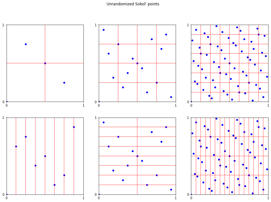
# unrandomized
fig,ax = pyplot.subplots(ncols=3,nrows=2,figsize=(15,10))
s = DigitalNetB2(2,randomize=False)
plt_ei(s.gen_samples(2**2,warn=False),ax[0,0],2,2)
plt_ei(s.gen_samples(2**3,warn=False),ax[1,0],8,0)
plt_ei(s.gen_samples(2**4,warn=False),ax[0,1],4,4)
plt_ei(s.gen_samples(2**4,warn=False),ax[1,1],2,8)
plt_ei(s.gen_samples(2**6,warn=False),ax[0,2],8,8)
plt_ei(s.gen_samples(2**6,warn=False),ax[1,2],16,4)
fig.suptitle("Unrandomized Sobol' points");
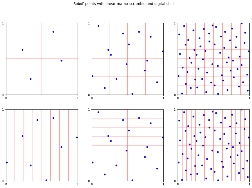
fig,ax = pyplot.subplots(ncols=3,nrows=2,figsize=(15,10))
s = DigitalNetB2(2,randomize='LMS_DS')
plt_ei(s.gen_samples(2**2,warn=False),ax[0,0],2,2)
plt_ei(s.gen_samples(2**3,warn=False),ax[1,0],8,0)
plt_ei(s.gen_samples(2**4,warn=False),ax[0,1],4,4)
plt_ei(s.gen_samples(2**4,warn=False),ax[1,1],2,8)
plt_ei(s.gen_samples(2**6,warn=False),ax[0,2],8,8)
plt_ei(s.gen_samples(2**6,warn=False),ax[1,2],16,4)
fig.suptitle("Sobol' points with linear matrix scramble and digital shift");
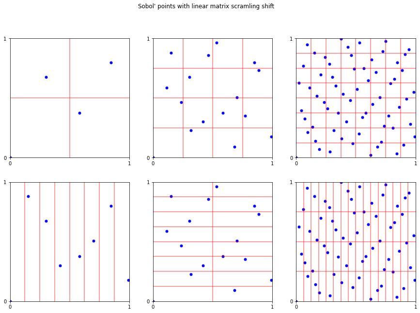
fig,ax = pyplot.subplots(ncols=3,nrows=2,figsize=(15,10))
s = DigitalNetB2(2,graycode=True,randomize='LMS')
plt_ei(s.gen_samples(2**2,warn=False),ax[0,0],2,2)
plt_ei(s.gen_samples(2**3,warn=False),ax[1,0],8,0)
plt_ei(s.gen_samples(2**4,warn=False),ax[0,1],4,4)
plt_ei(s.gen_samples(2**4,warn=False),ax[1,1],2,8)
plt_ei(s.gen_samples(2**6,warn=False),ax[0,2],8,8)
plt_ei(s.gen_samples(2**6,warn=False),ax[1,2],16,4)
fig.suptitle("Sobol' points with linear matrix scramling shift");
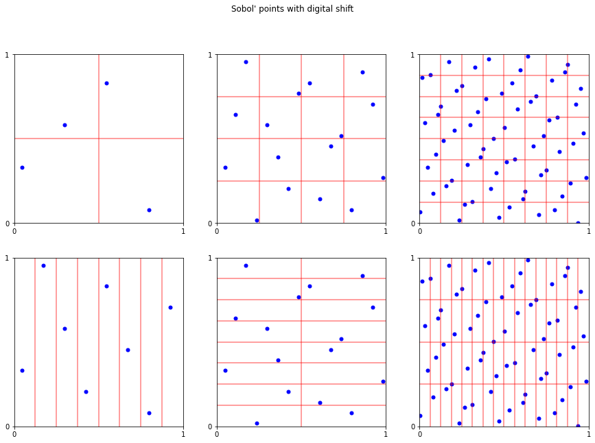
fig,ax = pyplot.subplots(ncols=3,nrows=2,figsize=(15,10))
s = DigitalNetB2(2,graycode=True,randomize='DS')
plt_ei(s.gen_samples(2**2,warn=False),ax[0,0],2,2)
plt_ei(s.gen_samples(2**3,warn=False),ax[1,0],8,0)
plt_ei(s.gen_samples(2**4,warn=False),ax[0,1],4,4)
plt_ei(s.gen_samples(2**4,warn=False),ax[1,1],2,8)
plt_ei(s.gen_samples(2**6,warn=False),ax[0,2],8,8)
plt_ei(s.gen_samples(2**6,warn=False),ax[1,2],16,4)
fig.suptitle("Sobol' points with digital shift");
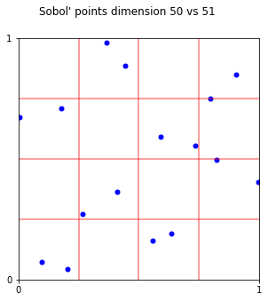
fig,ax = pyplot.subplots(figsize=(15,5))
s = DigitalNetB2([50,51],randomize='LMS_DS')
plt_ei(s.gen_samples(2**4),ax,4,4)
fig.suptitle("Sobol' points dimension 50 vs 51");
# nice properties do not necessary hold in higher dimensions
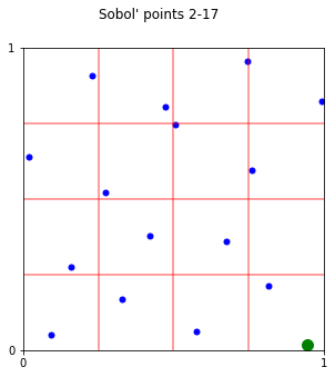
fig,ax = pyplot.subplots(figsize=(15,5))
s = DigitalNetB2(2,randomize='LMS_DS',graycode=True)
plt_ei(s.gen_samples(n_min=1,n_max=16),ax,4,4)
x16 = s.gen_samples(n_min=16,n_max=17)
ax.scatter(x16[:,0],x16[:,1],color='g',s=100)
fig.suptitle("Sobol' points 2-17");
# bbetter to take points 1-16 instead of 2-16
Skipping points vs. randomization
The first point in a Sobol’ sequence is  . Therefore, some
software packages skip this point as various transformations will map 0
to NAN. For example, the inverse CDF of a Gaussian density at
is
. Therefore, some
software packages skip this point as various transformations will map 0
to NAN. For example, the inverse CDF of a Gaussian density at
is  . However, we argue that it is better
to randomize points than to simply skip the first point for the
following reasons:
. However, we argue that it is better
to randomize points than to simply skip the first point for the
following reasons:
Skipping the first point does not give the uniformity advantages when taking powers of 2. For example, notice the green point in the above plot of “Sobol’ points 2-17”.
Randomizing Sobol’ points will return 0 with probability 0.
A more thorough explanation can be found in Art Owen’s paper On dropping the first Sobol’ point
So always randomize your Sobol’ unless you specifically need unrandomized points. In QMCPy the Sobol’ generator defaults to randomization with a linear matrix scramble.
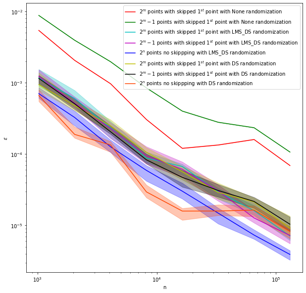
The below code runs tests comparing unrandomized vs. randomization with
linear matrix scramble with digital shift vs. randomization with just
digital shift. Furthermore, we compare taking the first  points vs. dropping the first point and taking points
vs. dropping the first point and taking
points vs. dropping the first point and taking points
vs. dropping the first point and taking  points.
N[Integrate[E^(-x1^2 - x2^2) Cos[Sqrt[x1^2 + x2^2]], {x1, -Infinity, Infinity}, {x2, -Infinity, Infinity}]]Plots the median (line) and fills the middle 10% of observations
def plt_k2d_sobol(ax,rtype,colors,plts=[1,2,3]):
    trials = 100
    solution = 1.808186429263620
    ms = arange(10,18)
    ax.set_xscale('log',base=2)
    ax.set_yscale('log',base=10)
    epsilons = {}
    if 1 in plts:
        epsilons['$2^m$ points with skipped $1^{st}$ point'] = zeros((trials,len(ms)),dtype=double)
    if 2 in plts:
        epsilons['$2^m-1$ points with skipped $1^{st}$ point'] = zeros((trials,len(ms)),dtype=double)
    if 3 in plts:
        epsilons['$2^n$ points no skippping'] = zeros((trials,len(ms)),dtype=double)
    for i,m in enumerate(ms):
        for t in range(trials):
            s = DigitalNetB2(2,randomize=rtype,graycode=True)
            k = Keister(s)
            if 1 in plts:
                epsilons['$2^m$ points with skipped $1^{st}$ point'][t,i] = \
                     abs(k.f(s.gen_samples(n_min=1,n_max=1+2**m)).mean()-solution)
            if 2 in plts:
                epsilons['$2^m-1$ points with skipped $1^{st}$ point'][t,i] = \
                     abs(k.f(s.gen_samples(n_min=1,n_max=2**m)).mean()-solution)
            if 3 in plts:
                epsilons['$2^n$ points no skippping'][t,i] = \
                     abs(k.f(s.gen_samples(n=2**m)).mean()-solution)
    for i,(label,eps) in enumerate(epsilons.items()):
        bot = percentile(eps, 40, axis=0)
        med = percentile(eps, 50, axis=0)
        top = percentile(eps, 60, axis=0)
        ax.loglog(2**ms,med,label=label+' with %s randomization'%rtype,color=colors[i])
        ax.fill_between(2**ms, bot, top, color=colors[i], alpha=.3)
# compare randomization fig,ax = pyplot.subplots(figsize=(10,10))
fig,ax = pyplot.subplots(figsize=(10,10))
plt_k2d_sobol(ax,None,['r','g'],[1,2])
plt_k2d_sobol(ax,'LMS_DS',['c','m','b'],[1,2,3])
plt_k2d_sobol(ax,'DS',['y','k','orangered'],[1,2,3])
ax.legend()
ax.set_xlabel('n')
ax.set_ylabel('$\\epsilon$');