Elliptic PDE

import copy
import numpy as np
import matplotlib as mpl
import matplotlib.pyplot as plt
from scipy.special import gamma, kv
from qmcpy.integrand._integrand import Integrand
from qmcpy.accumulate_data.mlmc_data import MLMCData
from qmcpy.accumulate_data.mlqmc_data import MLQMCData
import qmcpy as qp

# matplotlib options
rc_fonts = {
    "text.usetex": True,
    "font.size": 14,
    "mathtext.default": "regular",
    "axes.titlesize": 14,
    "axes.labelsize": 14,
    "legend.fontsize": 14,
    "xtick.labelsize": 12,
    "ytick.labelsize": 12,
    "figure.titlesize": 16,
    "font.family": "serif",
    "font.serif": "computer modern roman",
}
mpl.rcParams.update(rc_fonts)

# set random seed for reproducability
np.random.seed(9999)

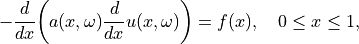
We will apply various multilevel Monte Carlo and multilevel quasi-Monte Carlo methods to approximate the expected value of a quantity of interest derived from the solution of a one-dimensional partial differential equation (PDE), where the diffusion coefficient of the PDE is a lognormal Gaussian random field. This example problem serves as an important benchmark problem for various methods in the uncertainty quantification and quasi-Monte Carlo literature. It is often referred to as the fruitfly problem of uncertainty quantification.

1. Problem definition

Let $Q$ be a quantity of interest derived from the solution $u(x, \omega)$ of the one-dimensional partial differential equation (PDE)

$-\frac{d}{dx}\bigg(a(x, \omega) \frac{d}{dx} u(x, \omega) \bigg) = f(x), \quad 0 \leq x \leq 1,$

$u(0, \cdot) = u_0,$

$u(1, \cdot) = u_1.$

The notation $u(x, \omega)$ is used to indicate that the solution depends on both the spatial variable $x$ and the uncertain parameter $\omega$ . This uncertainty is present because the diffusion coefficient, $a(x, \omega)$ , is given by a lognormal Gaussian random field with given covariance function. A common choice for the covariance function is the so-called Matérn covariance function

$c(x, y) = \hat{c}\bigg(\frac{\|x - y\|}{\lambda}\bigg)\quad \quad \hat{c}(r) = \frac{2^{1-\nu}}{\Gamma(\nu)} r^\nu K_\nu(r)$

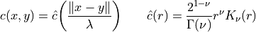
with $\Gamma$ the gamma function and $K_\nu$ the Bessel function of the second kind. This covariance function has two parameters: $\lambda$ , the length scale, and $\nu$ , the smoothness parameter.

We begin by defining the Matérn covariance function Matern(x, y):

def Matern(x, y, smoothness=1, lengthscale=1):
    distance = abs(x - y)
    r = distance/lengthscale
    prefactor = 2**(1-smoothness)/gamma(smoothness)
    term1 = r**smoothness
    term2 = kv(smoothness, r)
    np.fill_diagonal(term2, 1)
    cov = prefactor * term1 * term2
    np.fill_diagonal(cov, 1)
    return cov

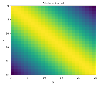
Let’s take a look at the covariance matrix obtained by evaluating the covariance function in n=25 equidistant points in [0, 1].

def get_covariance_matrix(pts, smoothness=1, lengthscale=1):
    X, Y = np.meshgrid(pts, pts)
    return Matern(X, Y, smoothness, lengthscale)

n = 25
pts = np.linspace(0, 1, num=n)
fig, ax = plt.subplots(figsize=(6, 5))
ax.pcolor(get_covariance_matrix(pts).T)
ax.invert_yaxis()
ax.set_ylabel(r"$x$")
ax.set_xlabel(r"$y$")
ax.set_title(f"Matern kernel")
plt.show()

A lognormal Gaussian random field $a(x, \omega)$ can be expressed as 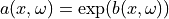$a(x, \omega) = \exp(b(x, \omega))$ , where $b(x, \omega)$ is a Gaussian random field. Samples of the Gaussian random field $b(x, \omega)$ can be computed from a factorization of the covariance matrix. Specifically, suppose we have a spectral (eigenvalue) expansion of the covariance matrix $C$ as

$C = V W V^T,$

then samples of the Gaussian random field can be computed as

$\boldsymbol{b} = S \boldsymbol{x},$

where $S = V W^{1/2}$ and $\boldsymbol{x}$ is a vector of standard normal independent and identically distributed random variables. This is easy to see, since

$\mathbb{E}[\boldsymbol{b}] = \mathbb{E}[S \boldsymbol{x}] = S\mathbb{E}[\boldsymbol{x}] = \boldsymbol{0}$

$\mathbb{E}[\boldsymbol{b} \boldsymbol{b}^T] = \mathbb{E}[S \boldsymbol{x} \boldsymbol{x}^T S^T] = S \mathbb{E}[\boldsymbol{x} \boldsymbol{x}^T] S^T = SS^T = VWV^T = C.$

First, let’s compute an eigenvalue decomposition of the covariance matrix.

def get_eigenpairs(n, smoothness=1, lengthscale=1):
    h = 1/(n-1)
    pts = np.linspace(h/2, 1 - h/2, num=n - 1)
    cov = get_covariance_matrix(pts, smoothness, lengthscale)
    w, v = np.linalg.eig(cov)
    # ensure all eigenvectors are correctly oriented
    for col in range(v.shape[1]):
        if v[0, col] < 0:
            v[:, col] *= -1
    return pts, w, v

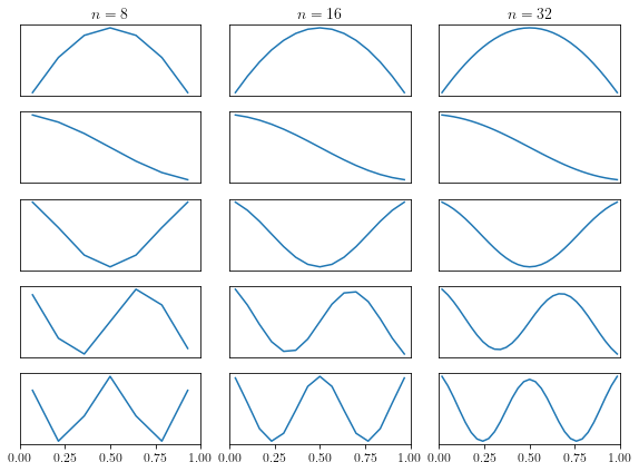
Next, we plot the eigenfunctions for different values of $n$ , the number of grid points.

n = [8, 16, 32] # list of number of gridpoints to plot
m = 5 # number of eigenfunctions to plot
fig, axes = plt.subplots(m, len(n), figsize=(8, 6))
for j, k in enumerate(n):
    x, w, v = get_eigenpairs(k)
    for i in range(m):
        axes[i, j].plot(x, v[:, i])
        axes[i, j].set_xlim(0, 1)
        axes[i, j].get_yaxis().set_ticks([])
        if i < m - 1:
            axes[i, j].get_xaxis().set_ticks([])
        if i == 0:
            axes[i, j].set_title(r"$n = " + repr(k) + r"$")
plt.tight_layout()

With this eigenvalue decomposition, we can compute samples of the Gaussian random field $b(x, \omega)$ , and hence, also of the lognormal Gaussian random field $a(x, \omega) = \exp(b(x, \omega))$ , since $\boldsymbol{b} = V W^{1/2} \boldsymbol{x}$ .

def evaluate(w, v, y=None):
    if y is None:
        y = np.random.randn(len(w) - 1)
    m = len(y)
    return v[:, :m] @ np.diag(np.sqrt(w[:m])) @ y

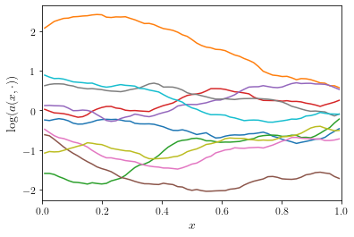
Let’s plot a couple of realizations of the Gaussian random field $b(x, \omega)$ .

n = 64
x, w, v = get_eigenpairs(n)
fig, ax = plt.subplots(figsize=(6, 4))
for _ in range(10):
    ax.plot(x, evaluate(w, v))
ax.set_xlim(0, 1)
ax.set_xlabel(r"$x$")
ax.set_ylabel(r"$\log(a(x, \cdot))$")
plt.show()

Now that we are able to compute realizations of the Gaussian random field, a next step is to compute a numerical solution of the PDE

$-\frac{d}{dx}\bigg(a(x, \omega) \frac{d}{dx} u(x, \omega) \bigg) = f(x), \quad 0 \leq x \leq 1.$

Using a straightforward finite-difference approximation, it is easy to show that the numerical solution $\boldsymbol{u}$ is the solution of a tridiagonal system. The solutions of such a tridiagonal system can be easily obtained in $O(n)$ (linear) time using the tridiagonal matrix algorithm (also known as the Thomas algorithm). More details can be found here.

def thomas(a, b, c, d):
    n = len(b)
    x = np.zeros(n)
    for i in range(1, n):
        w = a[i-1]/b[i-1]
        b[i] -= w*c[i-1]
        d[i] -= w*d[i-1]
    x[n-1] = d[n-1]/b[n-1]
    for i in reversed(range(n-1)):
        x[i] = (d[i] - c[i]*x[i+1])/b[i]
    return x

For the remainder of this notebook, we will assume that the source term $f(x)=1$ and Dirichlet boundary conditions $u(0) = u(1) = 0$ .

def pde_solve(a):
    n = len(a)
    b = np.full((n-1, 1), 1/n**2)
    x = thomas(-a[1:n-1], a[:n-1] + a[1:], -a[1:n-1], b)
    return np.insert(x, [0, n-1], [0, 0])

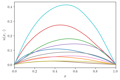
Let’s compute and plot a couple of solutions $u(x, \omega)$ .

n = 64
_, w, v = get_eigenpairs(n)
x = np.linspace(0, 1, num=n)
fig, ax = plt.subplots(figsize=(6, 4))
for _ in range(10):
    a = np.exp(evaluate(w, v))
    u = pde_solve(a)
    ax.plot(x, u)
ax.set_xlim(0, 1)
ax.set_xlabel(r"$x$")
ax.set_ylabel(r"$u(x, \cdot)$")
plt.show()

In the multilevel Monte Carlo method, we will rely on the ability to generate “correlated” solutions of the PDE with varying mesh sizes. Such a correlated solutions can be used as efficient control variates to reduce the variance (or statistical error) in the approximation of the expected value $\mathbb{E}[Q]$ . Since we are using a factorization of the covariance matrix to generate realizations of the Gaussian random field, it is quite easy to obtain correlated samples: when sampling from the “coarse” solution level, use the same set of random numbers used to sample from the “fine” solution level, but truncated to the appropriate size. Since the eigenvalue decomposition will reveal the most important modes in the covariance matrix, that same eigenvalue decomposition on a “coarse” approximation level will contain the same eigenfunctions, represented on the coarse grid. Let’s illustrate this property on an example using n = 16 grid points for the fine solution level and n = 8 grid points for the coarse solution level.

nf = 16
nc = nf//2
_, wf, vf = get_eigenpairs(nf)
_, wc, vc = get_eigenpairs(nc)
xf = np.linspace(0, 1, num=nf)
xc = np.linspace(0, 1, num=nc)
fig, ax = plt.subplots(figsize=(6, 4))
for _ in range(10):
    yf = np.random.randn(nf - 1)
    af = np.exp(evaluate(wf, vf, y=yf))
    uf = pde_solve(af)
    ax.plot(xf, uf)
    yc = yf[:nc - 1]
    ac = np.exp(evaluate(wc, vc, y=yc))
    uc = pde_solve(ac)
    ax.plot(xc, uc, color=ax.lines[-1].get_color(), linestyle="dashed", dash_capstyle="round")
ax.set_xlim(0, 1)
ax.set_ylim(bottom=0)
ax.set_xlabel(r"$x$")
ax.set_ylabel(r"$u(x, \cdot)$")
plt.show()

The better the coarse solution matches the fine grid solution, the more efficient the multilevel methods in Section 3 will perform.

2. Single-level methods

Let’s begin by using the single-level Monte Carlo and quasi-Monte Carlo methods to compute the expected value $\mathbb{E}[Q]$ . As quantity of interest $Q$ we take the solution of the PDE at $x=1/2$ , i.e., $Q = u(1/2, \cdot)$ .

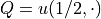To integrate the elliptic PDE problem into QMCPy, we construct a simple class as follows:

class EllipticPDE(Integrand):

    def __init__(self, sampler, smoothness=1, lengthscale=1):
        self.parameters = ["smoothness", "lengthscale", "n"]
        self.smoothness = smoothness
        self.lengthscale = lengthscale
        self.n = len(sampler.gen_samples(n=1)[0]) + 1
        self.compute_eigenpairs()
        self.sampler = sampler
        self.true_measure = qp.Gaussian(self.sampler)
        super(EllipticPDE, self).__init__(dimension_indv=1,dimension_comb=1,parallel=False)

    def compute_eigenpairs(self):
        _, w, v = get_eigenpairs(self.n)
        self.eigenpairs = w, v

    def g(self, x):
        n, d = x.shape
        return np.array([self.__g(x[j, :].T) for j in range(n)])

    def __g(self, x):
        w, v = self.eigenpairs
        a = np.exp(evaluate(w, v, y=x))
        u = pde_solve(a)
        return u[len(u)//2]

    def _spawn(self, level, sampler):
        return EllipticPDE(sampler, smoothness=self.smoothness, lengthscale=self.lengthscale)

# Custom print function
def print_data(data):
    for key, val in vars(data).items():
        kv = getattr(data, key)
        if hasattr(kv, "parameters"):
            print(f"{key}: {type(val).__name__}")
            for param in kv.parameters:
                print(f"\t{param}: {getattr(kv, param)}")
    for param in data.parameters:
        print(f"{param}: {getattr(data, param)}")

# Main function to test different methods
def test(problem, sampler, stopping_criterium, abs_tol=5e-3, verbose=True, **kwargs):
    integrand = problem(sampler)
    solution, data = stopping_criterium(integrand, abs_tol=abs_tol, **kwargs).integrate()
    if verbose:
        print(data)
        print("\nComputed solution %.3f in %.2f s"%(solution, data.time_integrate))

Next, let’s apply simple Monte Carlo to approximate the expected value $\mathbb{E}[Q]$ . The Monte Carlo estimator for $\mathbb{E}[Q]$ is simply the sample average over a finite set of samples, i.e.,

$\mathcal{Q}_N^\text{MC} := \frac{1}{N} \sum_{n=0}^{N-1} Q^{(n)},$

where $Q^{(n)} := u(1/2, \boldsymbol{x}^{(n)})$ and we explicitly denote the dependency of $Q$ on the standard normal random numbers $\boldsymbol{x}$ used to sample from the Gaussian random field. We will continue to increase the number of samples $N$ until a certain error criterion is satisfied.

# MC
test(EllipticPDE, qp.IIDStdUniform(32), qp.CubMCCLT)

MeanVarData (AccumulateData Object)
    solution        0.190
    error_bound     0.005
    n_total         19186
    n               18162
    levels          1
    time_integrate  4.307
CubMCCLT (StoppingCriterion Object)
    abs_tol         0.005
    rel_tol         0
    n_init          2^(10)
    n_max           10000000000
    inflate         1.200
    alpha           0.010
EllipticPDE (Integrand Object)
    smoothness      1
    lengthscale     1
    n               33
Gaussian (TrueMeasure Object)
    mean            0
    covariance      1
    decomp_type     PCA
IIDStdUniform (DiscreteDistribution Object)
    d               2^(5)
    entropy         326194454235761696154918970274080109080
    spawn_key       ()

Computed solution 0.190 in 4.31 s

The solution should be $\approx 0.189$ .

Similarly, the quasi-Monte Carlo estimator for $\mathbb{E}[Q]$ is defined as

$\mathcal{Q}_N^\text{QMC} := \frac{1}{N} \sum_{n=0}^{N-1} Q^{(n)},$

where $Q^{(n)} := u(1/2, \boldsymbol{t}^{(n)})$ with $\boldsymbol{t}^{(n)}$ the $n$ th low-discrepancy point transformed to the distribution of interest. For our elliptic PDE, this means that the quasi-Monte Carlo points, generated inside the unit cube $[0, 1)^d$ , are mapped to $\mathbb{R}^d$ .

Because the quasi-Monte Carlo estimator doesn’t come with a reliable error estimator, we run $K$ different quasi-Monte Carlo estimators in parallel. The sample variance over these $K$ different estimators can then be used as an error estimator.

# QMC
test(EllipticPDE, qp.Lattice(32), qp.CubQMCCLT, n_init=32)

MeanVarDataRep (AccumulateData Object)
    solution        0.189
    comb_bound_low  0.185
    comb_bound_high 0.192
    comb_flags      1
    n_total         2^(11)
    n               2^(11)
    n_rep           2^(7)
    time_integrate  0.490
CubQMCCLT (StoppingCriterion Object)
    inflate         1.200
    alpha           0.010
    abs_tol         0.005
    rel_tol         0
    n_init          2^(5)
    n_max           2^(30)
    replications    2^(4)
EllipticPDE (Integrand Object)
    smoothness      1
    lengthscale     1
    n               33
Gaussian (TrueMeasure Object)
    mean            0
    covariance      1
    decomp_type     PCA
Lattice (DiscreteDistribution Object)
    d               2^(5)
    dvec            [ 0  1  2 ... 29 30 31]
    randomize       1
    order           natural
    entropy         296354698279282161707952401923456574428
    spawn_key       ()

Computed solution 0.189 in 0.49 s

3. Multilevel methods

Implicit to the Monte Carlo and quasi-Monte Carlo methods above is a discretization parameter used in the numerical solution of the PDE. Let’s denote this parameter by $\ell$ , $0 \leq \ell \leq L$ . Multilevel methods are based on a telescopic sum expansion for the expected value $\mathbb{E}[Q_L]$ , as follows:

$\mathbb{E}[Q_L] = \mathbb{E}[Q_0] + \mathbb{E}[Q_1 - Q_0] + ... + \mathbb{E}[Q_L - Q_{L-1}].$

Using a Monte Carlo method for each of the terms on the right hand side yields a multilevel Monte Carlo method. Similarly, using a quasi-Monte Carlo method for each term on the right hand side yields a multilevel quasi-Monte Carlo method.

3.1 Multilevel (quasi-)Monte Carlo

Our class EllipticPDE needs some changes to be integrated with the multilevel methods in QMCPy.

class MLEllipticPDE(Integrand):

    def __init__(self, sampler, smoothness=1, lengthscale=1, _level=None):
        self.l = _level
        self.parameters = ["smoothness", "lengthscale", "n", "nb_of_levels"]
        self.smoothness = smoothness
        self.lengthscale = lengthscale
        dim = sampler.d + 1
        self.nb_of_levels = int(np.log2(dim + 1))
        self.n = [2**(l+1) + 1 for l in range(self.nb_of_levels)]
        self.compute_eigenpairs()
        self.sampler = sampler
        self.true_measure = qp.Gaussian(self.sampler)
        self.leveltype = "adaptive-multi"
        self.sums = np.zeros(6)
        self.cost = 0
        super(MLEllipticPDE, self).__init__(dimension_indv=1,dimension_comb=1,parallel=False)

    def _spawn(self, level, sampler):
        return MLEllipticPDE(sampler, smoothness=self.smoothness, lengthscale=self.lengthscale, _level=level)

    def compute_eigenpairs(self):
        self.eigenpairs = {}
        for l in range(self.nb_of_levels):
            _, w, v = get_eigenpairs(self.n[l])
            self.eigenpairs[l] = w, v

    def g(self, x): # This function is called by keyword reference for the level parameter "l"!
        n, d = x.shape

        Qf = np.array([self.__g(x[j, :].T, self.l) for j in range(n)])
        dQ = Qf
        if self.l > 0: # Compute multilevel difference
            dQ -= np.array([self.__g(x[j, :].T, self.l - 1) for j in range(n)])

        self.update_sums(dQ, Qf)
        self.cost = n*nf

        return dQ

    def __g(self, x, l):
        w, v = self.eigenpairs[l]
        n = self.n[l]
        a = np.exp(evaluate(w, v, y=x[:n-1]))
        u = pde_solve(a)
        return u[len(u)//2]

    def update_sums(self, dQ, Qf):
        self.sums[0] = dQ.sum()
        self.sums[1] = (dQ**2).sum()
        self.sums[2] = (dQ**3).sum()
        self.sums[3] = (dQ**4).sum()
        self.sums[4] = Qf.sum()
        self.sums[5] = (Qf**2).sum()

    def _dimension_at_level(self, l):
        return self.n[l]

Let’s apply multilevel Monte Carlo to the elliptic PDE problem.

test(MLEllipticPDE, qp.IIDStdUniform(32), qp.CubMCML)

MLMCData (AccumulateData Object)
    solution        0.191
    n_total         81898
    levels          3
    n_level         [31258.  5902.  4173.]
    mean_level      [1.901e-01 6.267e-04 1.575e-04]
    var_level       [5.150e-02 3.690e-04 9.224e-05]
    cost_per_sample [16. 16. 16.]
    alpha           1.993
    beta            2.000
    gamma           2^(-1)
    time_integrate  2.223
CubMCML (StoppingCriterion Object)
    rmse_tol        0.002
    n_init          2^(8)
    levels_min      2^(1)
    levels_max      10
    theta           2^(-1)
MLEllipticPDE (Integrand Object)
    smoothness      1
    lengthscale     1
    n               [ 3  5  9 17 33]
    nb_of_levels    5
Gaussian (TrueMeasure Object)
    mean            0
    covariance      1
    decomp_type     PCA
IIDStdUniform (DiscreteDistribution Object)
    d               2^(5)
    entropy         52139997603444977626041483839545508893
    spawn_key       ()

Computed solution 0.191 in 2.22 s

Now it’s easy to switch to multilevel quasi-Monte Carlo. Just change the discrete distribution from IIDStdUniform to Lattice.

test(MLEllipticPDE, qp.Lattice(32), qp.CubQMCML, n_init=32)

MLQMCData (AccumulateData Object)
    solution        0.190
    n_total         74752
    n_level         [2048.  256.   32.]
    levels          3
    mean_level      [ 1.900e-01  2.662e-05 -4.765e-05]
    var_level       [8.161e-07 4.455e-07 1.539e-07]
    bias_estimate   2.06e-04
    time_integrate  3.550
CubQMCML (StoppingCriterion Object)
    rmse_tol        0.002
    n_init          2^(5)
    n_max           10000000000
    replications    2^(5)
MLEllipticPDE (Integrand Object)
    smoothness      1
    lengthscale     1
    n               [ 3  5  9 17 33]
    nb_of_levels    5
Gaussian (TrueMeasure Object)
    mean            0
    covariance      1
    decomp_type     PCA
Lattice (DiscreteDistribution Object)
    d               2^(5)
    dvec            [ 0  1  2 ... 29 30 31]
    randomize       1
    order           natural
    entropy         119695915373660257480153154875270156239
    spawn_key       ()

Computed solution 0.190 in 3.55 s

3.2 Continuation multilevel (quasi-)Monte Carlo

In the continuation multilevel (quasi-)Monte Carlo method, we run the standard multilevel (quasi-)Monte Carlo method for a sequence of larger tolerances to obtain better estimates of the algorithmic parameters. The continuation multilevel heuristic will generally compute the same solution just a bit faster.

test(MLEllipticPDE, qp.IIDStdUniform(32), qp.CubMCMLCont)

MLMCData (AccumulateData Object)
    solution        0.185
    n_total         18182
    levels          2^(2)
    n_level         [16273.  1288.   337.   256.]
    mean_level      [1.863e-01 1.710e-04 7.073e-04 2.501e-04]
    var_level       [5.082e-02 3.083e-04 2.395e-05 9.872e-07]
    cost_per_sample [16. 16. 16. 16.]
    alpha           2^(-1)
    beta            4.143
    gamma           2^(-1)
    time_integrate  0.863
CubMCMLCont (StoppingCriterion Object)
    rmse_tol        0.002
    n_init          2^(8)
    levels_min      2^(1)
    levels_max      10
    n_tols          10
    tol_mult        1.668
    theta_init      2^(-1)
    theta           0.010
MLEllipticPDE (Integrand Object)
    smoothness      1
    lengthscale     1
    n               [ 3  5  9 17 33]
    nb_of_levels    5
Gaussian (TrueMeasure Object)
    mean            0
    covariance      1
    decomp_type     PCA
IIDStdUniform (DiscreteDistribution Object)
    d               2^(5)
    entropy         56767261736751958322904251045568279667
    spawn_key       ()

Computed solution 0.185 in 0.86 s

test(MLEllipticPDE, qp.Lattice(32), qp.CubQMCMLCont, n_init=32)

MLQMCData (AccumulateData Object)
    solution        0.189
    n_total         41984
    n_level         [1024.  256.   32.]
    levels          3
    mean_level      [ 1.891e-01  1.470e-04 -1.685e-04]
    var_level       [1.582e-06 7.087e-07 3.647e-07]
    bias_estimate   4.66e-04
    time_integrate  1.260
CubQMCMLCont (StoppingCriterion Object)
    rmse_tol        0.002
    n_init          2^(5)
    n_max           10000000000
    replications    2^(5)
    levels_min      2^(1)
    levels_max      10
    n_tols          10
    tol_mult        1.668
    theta_init      2^(-1)
    theta           0.058
MLEllipticPDE (Integrand Object)
    smoothness      1
    lengthscale     1
    n               [ 3  5  9 17 33]
    nb_of_levels    5
Gaussian (TrueMeasure Object)
    mean            0
    covariance      1
    decomp_type     PCA
Lattice (DiscreteDistribution Object)
    d               2^(5)
    dvec            [ 0  1  2 ... 29 30 31]
    randomize       1
    order           natural
    entropy         112259460192958188918668417604759964310
    spawn_key       ()

Computed solution 0.189 in 1.26 s

4. Convergence tests

Finally, we will run some convergence tests to see how these methods behave as a function of the error tolerance.

# Main function to test convergence for given problem
def test_convergence(problem, sampler, stopping_criterium, abs_tol=1e-3, verbose=True, smoothness=1, lengthscale=1, **kwargs):
    integrand = problem(sampler, smoothness=smoothness, lengthscale=lengthscale)
    stopping_crit = stopping_criterium(integrand, abs_tol=abs_tol, **kwargs)

    # get accumulate_data
    try:
        stopping_crit.data = MLQMCData(stopping_crit, stopping_crit.integrand, stopping_crit.true_measure, stopping_crit.discrete_distrib, stopping_crit.levels_min, stopping_crit.levels_max, stopping_crit.n_init, stopping_crit.replications)
    except:
        stopping_crit.data = MLMCData(stopping_crit, stopping_crit.integrand, stopping_crit.true_measure, stopping_crit.discrete_distrib, stopping_crit.levels_min, stopping_crit.n_init, -1., -1., -1.)

    # manually call "integrate()"
    tol = []
    n_samp = []
    for t in range(stopping_crit.n_tols):
        stopping_crit.rmse_tol = stopping_crit.tol_mult**(stopping_crit.n_tols-t-1)*stopping_crit.target_tol # update tol
        stopping_crit._integrate() # call _integrate()
        tol.append(copy.copy(stopping_crit.rmse_tol))
        n_samp.append(copy.copy(stopping_crit.data.n_level))

        if verbose:
            print("tol = {:5.3e}, number of samples = {}".format(tol[-1], n_samp[-1]))

    return tol, n_samp

# Execute the convergence test
def execute_convergence_test(smoothness=1, lengthscale=1):

    # Convergence test for MLMC
    tol_mlmc, n_samp_mlmc = test_convergence(MLEllipticPDE, qp.IIDStdUniform(32), qp.CubMCMLCont, verbose=False)

    # Convergence test for MLQMC
    tol_mlqmc, n_samp_mlqmc = test_convergence(MLEllipticPDE, qp.Lattice(32), qp.CubQMCMLCont, verbose=False, n_init=32)

    # Compute cost per level
    max_levels = max(max([len(n_samp) for n_samp in n_samp_mlmc]), max([len(n_samp) for n_samp in n_samp_mlqmc]))
    cost_per_level = np.array([2**level + int(2**(level-1)) for level in range(max_levels)])
    cost_per_level = cost_per_level/cost_per_level[-1]

    # Compute total cost for each tolerance and store the result
    cost = {}
    cost["mc"] = (tol_mlmc, [n_samp_mlmc[tol][0] for tol in range(len(tol_mlmc))]) # where we assume V[Q_0] = V[Q_L]
    cost["qmc"] = (tol_mlqmc, [n_samp_mlqmc[tol][0] for tol in range(len(tol_mlqmc))]) # where we assume V[Q_0] = V[Q_L]
    cost["mlmc"] = (tol_mlmc, [sum([n_samp*cost_per_level[j] for j, n_samp in enumerate(n_samp_mlmc[tol])]) for tol in range(len(tol_mlmc))])
    cost["mlqmc"] = (tol_mlqmc, [sum([n_samp*cost_per_level[j] for j, n_samp in enumerate(n_samp_mlqmc[tol])]) for tol in range(len(tol_mlqmc))])

    return cost

# Plot the result
def plot_convergence(cost):
    fig, ax = plt.subplots(figsize=(8, 6))
    ax.plot(cost["mc"][0], cost["mc"][1], marker="o", label="MC")
    ax.plot(cost["qmc"][0], cost["qmc"][1], marker="o", label="QMC")
    ax.plot(cost["mlmc"][0], cost["mlmc"][1], marker="o", label="MLMC")
    ax.plot(cost["mlqmc"][0], cost["mlqmc"][1], marker="o", label="MLQMC")
    ax.legend(frameon=False)
    ax.set_xscale("log")
    ax.set_yscale("log")
    ax.set_xlabel(r"error tolerance $\varepsilon$")
    ax.set_ylabel(r"equivalent \# model evaluations at finest level")
    plt.show()

This command takes a while to execute (about 1 minute on my laptop):

plot_convergence(execute_convergence_test())

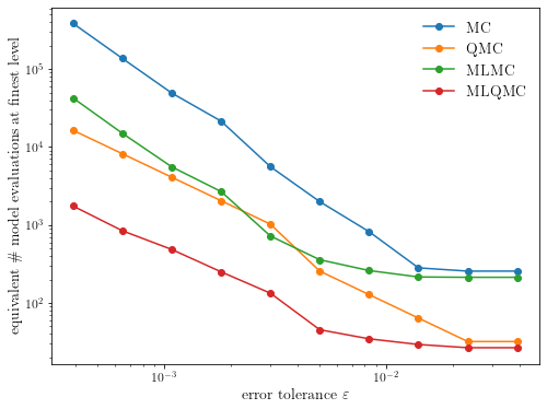
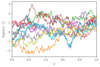
The benefit of the low-discrepancy point set depends on the smoothness of the random field: the smoother the random field, the better. Here’s an example for a Gaussian random field with a smaller smoothness $\nu=1/2$ and smaller length scale $\lambda=1/3$ .

smoothness = 1/2
lengthscale = 1/3

n = 256
x, w, v = get_eigenpairs(n, smoothness=smoothness, lengthscale=lengthscale)
fig, ax = plt.subplots(figsize=(6, 4))
for _ in range(10):
    ax.plot(x, evaluate(w, v))
ax.set_xlim(0, 1)
ax.set_xlabel(r"$x$")
ax.set_ylabel(r"$\log(a(x, \cdot))$")
plt.show()

plot_convergence(execute_convergence_test(lengthscale=lengthscale, smoothness=smoothness))

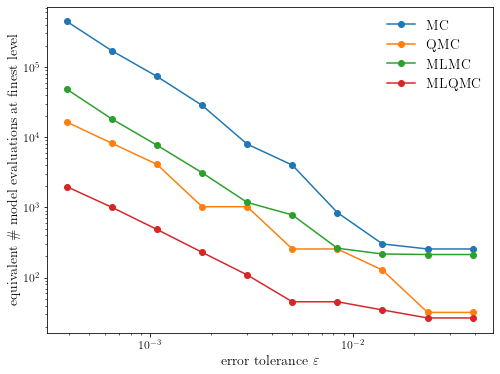
While the multilevel quasi-Monte Carlo method is still the fastest method, the asymptotic cost complexity of the QMC-based methods reduces to approximately the same rate as the MC-based methods.

The benefits of the multilevel methods over single-level methods will be even larger for two- or three-dimensional PDE problems, since it will be even more computationally efficient to take samples on a coarse grid.