Challenges in Developing Great QMC Software
Computations and Figures for the MCQMC 2022 Article: Challenges in Developing Great Quasi-Monte Carlo Software
Import the necessary packages and set up plotting routines
import matplotlib.pyplot as plt
import numpy as np
import qmcpy as qp
import time  #timing routines
import warnings  #to suppress warnings when needed
import pickle  #write output to a file and load it back in
from copy import deepcopy

plt.rc('font', size=16)  #set defaults so that the plots are readable
plt.rc('axes', titlesize=16)
plt.rc('axes', labelsize=16)
plt.rc('xtick', labelsize=16)
plt.rc('ytick', labelsize=16)
plt.rc('legend', fontsize=16)
plt.rc('figure', titlesize=16)

#a helpful plotting method to show increasing numbers of points
def plot_successive_points(distrib,ld_name,first_n=64,n_cols=1,
                           pt_clr=['tab:blue', 'tab:green', 'k', 'tab:cyan', 'tab:purple', 'tab:orange'],
                           xlim=[0,1],ylim=[0,1]):
  fig,ax = plt.subplots(nrows=1,ncols=n_cols,figsize=(5*n_cols,5.5))
  if n_cols==1: ax = [ax]
  last_n = first_n*(2**n_cols)
  points = distrib.gen_samples(n=last_n)
  for i in range(n_cols):
    n = first_n
    nstart = 0
    for j in range(i+1):
      n = first_n*(2**j)
      ax[i].scatter(points[nstart:n,0],points[nstart:n,1],color=pt_clr[j])
      nstart = n
    ax[i].set_title('n = %d'%n)
    ax[i].set_xlim(xlim); ax[i].set_xticks(xlim); ax[i].set_xlabel('$x_{i,1}$')
    ax[i].set_ylim(ylim); ax[i].set_yticks(ylim); ax[i].set_ylabel('$x_{i,2}$')
    ax[i].set_aspect((xlim[1]-xlim[0])/(ylim[1]-ylim[0]))
  fig.suptitle('%s Points'%ld_name, y=0.9)
  return fig

print('QMCPy Version',qp.__version__)
QMCPy Version 1.3.2
Make sure that you have the relevant path to store the figures
figpath = '' #this path sends the figures to the desired directory
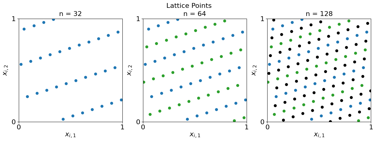
Here are some plots of Low Discrepancy (LD) Lattice Points
d = 5 #dimension
n = 32 #number of points
cols = 3 #number of columns
ld = qp.Lattice(d) #define the generator
fig = plot_successive_points(ld,'Lattice',first_n=n,n_cols=cols)
fig.savefig(figpath+'latticepts.eps',format='eps',bbox_inches='tight')
Beam Example Plots
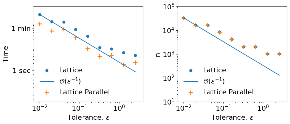
Plot the time and sample size required to solve for the deflection of the whole beam using low discrepancy with and without parallel
with open(figpath+'ld_parallel.pkl','rb') as myfile: tol_vec,n_tol,ld_time,ld_n,ld_p_time,ld_p_n,best_solution = pickle.load(myfile)
print(best_solution)
fig,ax = plt.subplots(nrows=1,ncols=2,figsize=(11,4))
ax[0].scatter(tol_vec[0:n_tol],ld_time[0:n_tol],color='tab:blue');
ax[0].plot(tol_vec[0:n_tol],[(ld_time[0]*tol_vec[0])/tol_vec[jj] for jj in range(n_tol)],color='tab:blue')
ax[0].scatter(tol_vec[0:n_tol],ld_p_time[0:n_tol],color='tab:orange',marker = '+',s=100,linewidths=2);
#ax[0].plot(tol_vec[0:n_tol],[(ld_p_time[0]*tol_vec[0])/tol_vec[jj] for jj in range(n_tol)],color='tab:orange')
ax[0].set_ylim([0.05,500]); ax[0].set_ylabel('Time')
ax[1].scatter(tol_vec[0:n_tol],ld_n[0:n_tol],color='tab:blue');
ax[1].plot(tol_vec[0:n_tol],[(ld_n[0]*tol_vec[0])/tol_vec[jj] for jj in range(n_tol)],color='tab:blue')
ax[1].scatter(tol_vec[0:n_tol],ld_p_n[0:n_tol],color='tab:orange',marker = '+',s=100,linewidths=2);
#ax[1].plot(tol_vec[0:n_tol],[(ld_p_n[0]*tol_vec[0])/tol_vec[jj] for jj in range(n_tol)],color='tab:orange')
ax[1].set_ylim([10,1e5]); ax[1].set_ylabel('n')
for ii in range(2):
  ax[ii].set_xlim([0.007,4]); ax[ii].set_xlabel('Tolerance, '+r'$\varepsilon$')
  ax[ii].set_xscale('log'); ax[ii].set_yscale('log')
  ax[ii].legend(['Lattice',r'$\mathcal{O}(\varepsilon^{-1})$','Lattice Parallel',r'$\mathcal{O}(\varepsilon^{-1})$'],frameon=False)
  ax[ii].set_aspect(0.6)
ax[0].set_yticks([1, 60], labels = ['1 sec', '1 min'])
fig.savefig(figpath+'ldparallelbeam.eps',format='eps',bbox_inches='tight')
[   0.            4.09650336   15.63089718   33.92196588   58.36259037
   88.42166624  123.63753779  163.62564457  208.07398743  256.74371736
  309.46852588  362.17337763  410.80019812  455.47543786  496.40155276
  533.85794874  568.20201672  599.87051305  629.38039738  657.32920342
  684.39496877  712.15829288  742.93687638  776.09146089  811.06031655
  847.35856113  884.57752606  922.38415394  960.52038491  998.8025606
 1037.12106673]
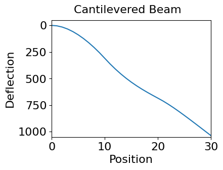
Plot of beam solution
fig,ax = plt.subplots(figsize=(6,3))
ax.plot(best_solution,'-')
ax.set_xlim([0,len(best_solution)-1]); ax.set_xlabel('Position')
ax.set_ylim([1050,-50]);  ax.set_ylabel('Deflection');
ax.set_aspect(0.02)
fig.suptitle('Cantilevered Beam')
fig.savefig(figpath+'cantileveredbeamwords.eps',format='eps',bbox_inches='tight')
qp.util.stop_notebook()
Type 'yes' to continue running notebookno
An exception has occurred, use %tb to see the full traceback.


SystemExit: Pausing notebook execution
Below is long-running code, that we rarely wish to run
Beam Example Computations
To run this, you need to be running the docker application,
https://www.docker.com/products/docker-desktop/
Set up the problem using a docker container to solve the ODE
import umbridge #this is the connector
!docker run --name muqbp -d -it -p 4243:4243 linusseelinger/benchmark-muq-beam-propagation:latest #get beam example
d = 3 #dimension of the randomness
lb = 1 #lower bound on randomness
ub = 1.2 #upper bound on randomness
umbridge_config = {"d": d}
model = umbridge.HTTPModel('http://localhost:4243','forward') #this is the original model
outindex = -1 #choose last element of the vector of beam deflections
modeli = deepcopy(model) #and construct a model for just that deflection
modeli.get_output_sizes = lambda *args : [1]
modeli.get_output_sizes()
modeli.__call__ = lambda *args,**kwargs: [[model.__call__(*args,**kwargs)[0][outindex]]]
docker: Error response from daemon: Conflict. The container name "/muqbp" is already in use by container "7f9e0237bd3e72783743efb67f78ce8cc800f5a24835f4191bc423f960cdedac". You have to remove (or rename) that container to be able to reuse that name.
See 'docker run --help'.
First we compute the time required to solve for the deflection of the end point using IID and low discrepancy
ld = qp.Uniform(qp.Lattice(d,seed=7),lower_bound=lb,upper_bound=ub) #lattice points for this problem
ld_integ = qp.UMBridgeWrapper(ld,modeli,umbridge_config,parallel=False) #integrand
iid = qp.Uniform(qp.IIDStdUniform(d),lower_bound=lb,upper_bound=ub) #iid points for this problem
iid_integ = qp.UMBridgeWrapper(iid,modeli,umbridge_config,parallel=False) #integrand
tol = 0.01  #smallest tolerance

n_tol = 14  #number of different tolerances
ii_iid = 9  #make this larger to reduce the time required by not running all cases for IID
tol_vec = [tol*(2**ii) for ii in range(n_tol)]  #initialize vector of tolerances
ld_time = [0]*n_tol; ld_n = [0]*n_tol  #low discrepancy time and number of function values
iid_time = [0]*n_tol; iid_n = [0]*n_tol  #IID time and number of function values
print(f'\nCantilever Beam\n')
print('iteration ', end = '')
for ii in range(n_tol):
  solution, data = qp.CubQMCLatticeG(ld_integ, abs_tol = tol_vec[ii]).integrate()
  if ii == 0:
    best_solution_i = solution
  ld_time[ii] = data.time_integrate
  ld_n[ii] = data.n_total
  if ii >= ii_iid:
    solution, data = qp.CubMCG(iid_integ, abs_tol = tol_vec[ii]).integrate()
    iid_time[ii] = data.time_integrate
    iid_n[ii] = data.n_total
  print(ii, end = ' ')
with open(figpath+'iid_ld.pkl','wb') as myfile:pickle.dump([tol_vec,n_tol,ii_iid,ld_time,ld_n,iid_time,iid_n,best_solution_i],myfile)
Cantilever Beam

iteration 0 1 2 3 4 5 6 7 8 9 10 11 12 13
Next, we compute the time required to solve for the deflection of the whole beam using low discrepancy with and without parallel
ld_integ = qp.UMBridgeWrapper(ld,model,umbridge_config,parallel=False) #integrand
ld_integ_p = qp.UMBridgeWrapper(ld,model,umbridge_config,parallel=8) #integrand with parallel processing

tol = 0.01
n_tol = 9  #number of different tolerances
tol_vec = [tol*(2**ii) for ii in range(n_tol)]  #initialize vector of tolerances
ld_time = [0]*n_tol; ld_n = [0]*n_tol  #low discrepancy time and number of function values
ld_p_time = [0]*n_tol; ld_p_n = [0]*n_tol  #low discrepancy time and number of function values with parallel
print(f'\nCantilever Beam\n')
print('iteration ', end = '')
for ii in range(n_tol):
  solution, data = qp.CubQMCLatticeG(ld_integ, abs_tol = tol_vec[ii]).integrate()
  if ii == 0:
    best_solution = solution
  ld_time[ii] = data.time_integrate
  ld_n[ii] = data.n_total
  solution, data = qp.CubQMCLatticeG(ld_integ_p, abs_tol = tol_vec[ii]).integrate()
  ld_p_time[ii] = data.time_integrate
  ld_p_n[ii] = data.n_total
  print(ii, end = ' ')
with open(figpath+'ld_parallel.pkl','wb') as myfile:pickle.dump([tol_vec,n_tol,ld_time,ld_n,ld_p_time,ld_p_n,best_solution],myfile)
Cantilever Beam

iteration 0 1 2 3 4 5 6 7 8
!docker rm -f muqbp #shut down docker image
